Content from Before we Start
Last updated on 2024-03-12 | Edit this page
Overview
Questions
- What is R and why learn it?
- How to find your way around RStudio?
- How to interact with R?
- How to install packages?
Objectives
- Navigate the RStudio interface.
- Install additional packages using the packages tab.
- Install additional packages using R code.
This episode is adapted from Before We Start from the R for Social Scientists Carpentry lesson, licensed under a Creative Commons Attribution 4.0 License (CC BY 4.0).
What is R? What is RStudio?
R is more of a programming language than just a
statistics program. It was started by Robert Gentleman and Ross Ihaka
from the University of Auckland in 1995. They described it as “a language
for data analysis and graphics.” You can use R to create, import, and
scrape data from the web; clean and reshape it; visualize it; run
statistical analysis and modeling operations on it; text and data mine
it; and much more. The term “R” is used to refer to both
the programming language and the software that interprets the scripts
written using it.
RStudio is a user interface for working with R. It is called an Integrated Development Environment (IDE): a piece of software that provides tools to make programming easier. RStudio acts as a sort of wrapper around the R language. You can use R without RStudio, but it’s much more limiting. RStudio makes it easier to import datasets, create and write scripts, and makes using R much more effective. RStudio is also free and open source. To function correctly, RStudio needs R and therefore both need to be installed on your computer.
Why learn R?
R does not involve lots of pointing and clicking, and that’s a good thing
The learning curve might be steeper than with other software, but with R, the results of your analysis do not rely on remembering a succession of pointing and clicking, but instead on a series of written commands, and that’s a good thing! So, if you want to redo your analysis because you collected more data, you don’t have to remember which button you clicked in which order to obtain your results; you just have to run your script again.
Working with scripts makes the steps you used in your analysis clear, and the code you write can be inspected by someone else who can give you feedback and spot mistakes. It forces you to have a deeper understanding of what you are doing, and facilitates your learning and comprehension of the methods you use.
R code is great for reproducibility
Reproducibility is when someone else (including your future self) can obtain the same results from the same dataset when using the same analysis.
R integrates with other tools to generate manuscripts from your code. If you collect more data, or fix a mistake in your dataset, the figures and the statistical tests in your manuscript are updated automatically.
An increasing number of journals and funding agencies expect analyses to be reproducible, so knowing R will give you an edge with these requirements.
R is interdisciplinary and extensible
With 10,000+ packages that can be installed to extend its capabilities, R provides a framework that allows you to combine statistical approaches from many scientific disciplines to best suit the analytical framework you need to analyze your data. For instance, R has packages for image analysis, GIS, time series, population genetics, and a lot more.
R works on data of all shapes and sizes
The skills you learn with R scale easily with the size of your dataset. Whether your dataset has hundreds or millions of lines, it won’t make much difference to you.
R is designed for data analysis. It comes with special data structures and data types that make handling of missing data and statistical factors convenient.
R can connect to spreadsheets, databases, and many other data formats, on your computer or on the web.
R produces high-quality graphics
The plotting functionalities in R are endless, and allow you to adjust any aspect of your graph to convey most effectively the message from your data.
R has a large and welcoming community
Thousands of people use R daily. Many of them are willing to help you through mailing lists and websites such as Stack Overflow, or on the RStudio community. Questions which are backed up with short, reproducible code snippets are more likely to attract knowledgeable responses.
Not only is R free, but it is also open-source and cross-platform
R is also free and open source, distributed under the terms of the GNU General Public License.. This means it is free to download and use the software for any purpose, modify it, and share it. Anyone can inspect the source code to see how R works. Because of this transparency, there is less chance for mistakes, and if you (or someone else) find some, you can report and fix bugs. As a result, R users have created thousands of packages and software to enhance user experience and functionality.
Because R is open source and is supported by a large community of developers and users, there is a very large selection of third-party add-on packages which are freely available to extend R’s native capabilities.

R and librarianship
For at least the last decade, librarians have been grappling with the ways that the “data deluge” affects our work on multiple levels–collection development, analyzing usage of the library website/space/collections, reference services, information literacy instruction, research support, accessing bibliographic metadata from third parties, and more.
By using R or any advanced data analysis platform (such as Python), libraries can harness data in order to:
- Clean messy data from the ILS & vendors
- Clean ISBNs, ISSNs, other identifiers
- Detect data errors & anomalies
- Normalize names (e.g. databases, ebooks, serials)
- Create custom subsets
- Merge and analyze data, e.g.
- Holdings and usage data from the same vendor
- Print book & ebook holdings
- COUNTER statistics
- Institutional data
- Recode variables
- Manipulate dates and times
- Create visualizations
- Provide data reference services
- Access data via APIs, including Crossref, Unpaywall, ORCID, and Sherpa-ROMeO
- Write documents to communicate findings
Knowing your way around RStudio
Let’s start by learning about RStudio, which is an Integrated Development Environment (IDE) for working with R.
The RStudio IDE open-source product is free under the Affero General Public License (AGPL) v3. The RStudio IDE is also available with a commercial license and priority email support from RStudio, Inc.
We will use the RStudio IDE to write code, navigate the files on our computer, inspect the variables we create, and visualize the plots we generate. RStudio can also be used for other things (e.g., version control, developing packages, writing Shiny apps) that we will not cover during the workshop.
One of the advantages of using RStudio is that all the information you need to write code is available in a single window. Additionally, RStudio provides many shortcuts, autocompletion, and highlighting for the major file types you use while developing in R. RStudio makes typing easier and less error-prone.
Getting set up
It is good practice to keep a set of related data, analyses, and text self-contained in a single folder called the working directory. All of the scripts within this folder can then use relative paths to files. Relative paths indicate where inside the project a file is located (as opposed to absolute paths, which point to where a file is on a specific computer). Working this way makes it a lot easier to move your project around on your computer and share it with others without having to directly modify file paths in the individual scripts.
RStudio provides a helpful set of tools to do this through its “Projects” interface, which not only creates a working directory for you but also remembers its location (allowing you to quickly navigate to it). The interface also (optionally) preserves custom settings and open files to make it easier to resume work after a break.
Create a new project
- Under the
Filemenu, click onNew project, chooseNew directory, thenNew project - Enter the name
library_carpentryfor this new folder (or “directory”). This will be your working directory for the rest of the day. - Click on
Create project - Create a new file where we will type our scripts. Go to File >
New File > R script. Click the save icon on your toolbar and save
your script as “
script.R”.
The RStudio Interface
Let’s take a quick tour of RStudio.
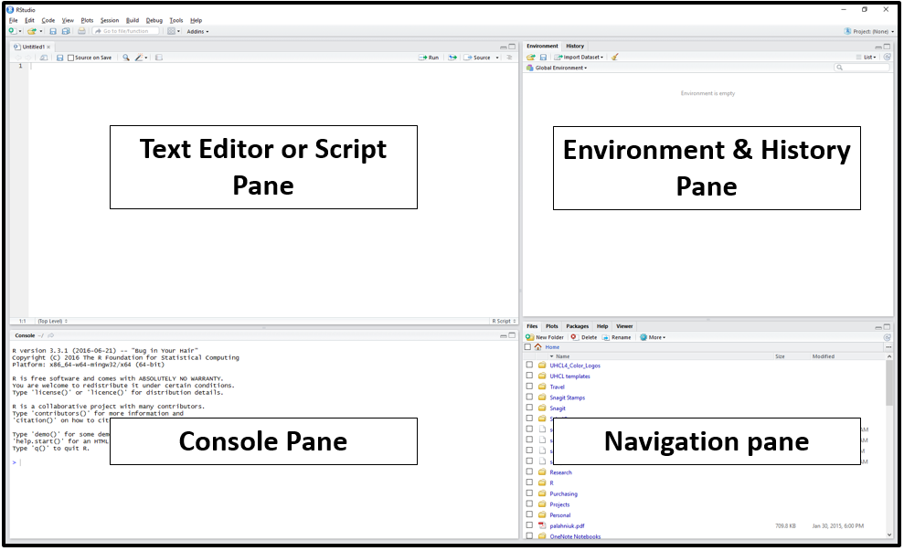
RStudio is divided into four “panes”. The placement of these panes and their content can be customized (see menu, Tools -> Global Options -> Pane Layout).
The Default Layout is:
Console Pane (bottom left) If you were just using the basic R interface, without RStudio, this is all you would see. You use this to type in a command and press enter to immediately evaluate it. It includes a
>symbol and a blinking cursor prompting you to enter some code. Code that you type directly in the console will not be saved, though it is available in the History Pane. You can try it out by typing2 + 2into the console.Script Pane (top left) This is sort of like a text editor, or a place to draft and save code. You then tell RStudio to run the line of code, or multiple lines of code, and you can see it appear in the console as it is running. Then save the script as a .R file for future use, or to share with others.
Environment/History Pane (top right) This will display the objects that you’ve read into what is called the “global environment.” When you read a file into R, or manually create an R object, it enters into the computer’s working memory. When we manipulate or run operations on that data, it isn’t written to a file until we tell it to. It is kept here in the RStudio environment. The History tab displays all commands that have been executed in the console.
-
Navigation Pane (bottom right) This pane has multiple functions:
- Files: Navigate to files saved on your computer and in your working directory
- Plots: View plots (e.g. charts and graphs) you have created
- Packages: view add-on packages you have installed, or install new packages
- Help: Read help pages for R functions
- Viewer: View local web content
Interacting with R
The basis of programming is that we write down instructions for the computer to follow, and then we tell the computer to follow those instructions. We write, or code, instructions in R because it is a common language that both the computer and we can understand.
There are two main ways of interacting with R: by using the console or by using script files (plain text files that contain your code). The console pane (in RStudio, the bottom left panel) is the place where commands written in the R language can be typed and executed immediately by the computer. It is also where the results will be shown for commands that have been executed. You can type commands directly into the console and press Enter to execute those commands, but they will be forgotten when you close the session.
The prompt is the blinking cursor in the console pane
prompting you to take action, in the lower-left corner of R Studio. If R
is ready to accept commands, the R console shows a >
prompt. If R receives a command (by typing, copy-pasting, or sent from
the script editor using Ctrl + Enter), R will try
to execute it and, when ready, will show the results and come back with
a new > prompt to wait for new commands. We type
commands into the prompt, and press the Enter key to
evaluate (also called execute or run) those
commands.
You can use R like a calculator:
R
2 + 2 # Type 2 + 2 in the console to run the command
While in the console, you can press the up and down keys on your keyboard to cycle through previously executed commands.
Because we want our code and workflow to be reproducible, it is better to type the commands we want in the script editor and save the script. This way, there is a complete record of what we did, and anyone (including our future selves!) can easily replicate the results on their computer.
RStudio allows you to execute commands directly from the script editor by using the Ctrl + Enter shortcut (on Mac, Cmd + Return will work). The command on the current line in the script (indicated by the cursor) or all of the commands in selected text will be sent to the console and executed when you press Ctrl + Enter. If there is information in the console you do not need anymore, you can clear it with Ctrl + L. You can find other keyboard shortcuts in this RStudio cheatsheet about the RStudio IDE.
At some point in your analysis, you may want to check the content of a variable or the structure of an object without necessarily keeping a record of it in your script. You can type these commands and execute them directly in the console. RStudio provides the Ctrl + 1 and Ctrl + 2 shortcuts allow you to jump between the script and the console panes.
If R is still waiting for you to enter more text, the console will
show a + prompt. It means that you haven’t finished
entering a complete command. This is likely because you have not
‘closed’ a parenthesis or quotation, i.e. you don’t have the same number
of left-parentheses as right-parentheses or the same number of opening
and closing quotation marks. When this happens, and you thought you
finished typing your command, click inside the console window andx press
Esc; this will cancel the incomplete command and return you
to the > prompt. You can then proofread the command(s)
you entered and correct the error.
Installing additional packages using the packages tab
When you download R it already has a number of functions built in:
these encompass what is called Base R. However, many R
users write their own libraries of functions, package
them together in R Packages, and provide them to the R
community at no charge. This extends the capacity of R and allows us to
do much more. In many cases, they improve on the Base R functions by
making them easier and more straightforward to use. In the course of
this lesson we will be making use of several of these packages, such as
ggplot2 and dplyr.
The Comprehensive R Archive Network (CRAN) is the main repository for R packages, and that organization maintains strict standards in order for a package to be listed–for example, it must include clear descriptions of the functions, and it must not track or tamper with the user’s R session. See this page from RStudio for a good list of useful R packages. In addition to CRAN, R users can make their code and packages available from GitHub. Finally, some communities host their own collections of R packages, such as Bioconductor for computational biology and bioinformatics.
Installing Packages
Installing CRAN packages can be done from the RStudio console. Click
the Packages tab in the Navigation Pane, then click Install and search
for the package you’re looking for. You can also use the
install.packages() function directly in the console. Run
help(install.packages) to learn more about how to do it
this way.
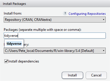
At the bottom of the Install Packages window is a check box to ‘Install’ dependencies. This is ticked by default, which is usually what you want. Packages can (and do) make use of functionality built into other packages, so for the functionality contained in the package you are installing to work properly, there may be other packages which have to be installed with them. The ‘Install dependencies’ option makes sure that this happens.
From the packages tab, click ‘Install’ from the toolbar and type ‘tidyverse’ into the textbox, then click ‘install’. The ‘tidyverse’ package is really a package of packages, including ‘ggplot2’ and ‘dplyr’, both of which require other packages to run correctly. All of these packages will be installed automatically. Depending on what packages have previously been installed in your R environment, the install of ‘tidyverse’ could be very quick or could take several minutes. As the install proceeds, messages relating to its progress will be written to the console. You will be able to see all of the packages which are actually being installed.
Because the install process accesses the CRAN repository, you will need an Internet connection to install packages.
It is also possible to install packages from other repositories, as well as Github or the local file system, but we won’t be looking at these options in this lesson.
Installing additional packages using R code
If you were watching the console window when you started the install of ‘tidyverse’, you may have noticed that the line
R
install.packages("tidyverse")
was written to the console before the start of the installation messages.
You could also have installed the
tidyverse packages by running this command
directly in the R console.
R Resources
Learning R
swirlis a package you can install in R to learn about R and data science interactively. Just typeinstall.packages("swirl")into your R console, load the package by typinglibrary("swirl"), and then typeswirl(). Read more at swirl.Try R is a browser-based interactive tutorial developed by Code School.
Anthony Damico’s twotorials are a series of 2 minute videos demonstrating several basic tasks in R.
Cookbook for R by Winston Change provides solutions to common tasks and problems in analyzing data.
If you’re up for a challenge, try the free R Programming MOOC in Coursera by Roger Peng.
Books:
- R For Data Science by Garrett Grolemund & Hadley Wickham [free]
- An Introduction to Data Cleaning with R by Edwin de Jonge & Mark van der Loo [free]
- YaRrr! The Pirate’s Guide to R by Nathaniel D. Phillips [free]
- Springer’s Use R! series [not free] is mostly specialized, but it has some excellent introductions including Alain F. Zuur et al.’s A Beginner’s Guide to R and Phil Spector’s Data Manipulation in R.
Data
If you need some data to play with, type data() in the
console for a list of data sets. To load a dataset, type it like this:
data(mtcars). Type help(mtcars) to learn more
about it. You can then perform operations, e.g.
R
head(mtcars)
nrow(mtcars)
mean(mtcars$mpg)
sixCylinder <- mtcars[mtcars$cyl == 6, ]
See also rdatamining.com’s list of free datasets.
Cheat Sheets
- Base R Cheat Sheet by Mhairi McNeill
- Data Transformation with dplyr Cheat Sheet by RStudio
- Data Wrangling with dplyr and tidyr Cheat Sheet by RStudio
- Complete list of RStudio cheatsheets
Style guides
Use these resources to write cleaner code, according to established style conventions
- Hadley Wickham’s Style Guide
- Google’s R Style Guide
- Tip: highlight code in your script pane and press Ctrl/Cmd + I on your keyboard to automatically fix the indents
Credit
Parts of this episode have been inspired by the following:
- “Before We Start” R for Social Scientists Carpentry Lesson. CC BY 4.0.
- Roger Peng’s Computing for Data Analysis videos
- Lisa Federer’s Introduction to R for Non-Programmers
- Brad Boehmke’s Intro to R Bootcamp
Content from Introduction to R
Last updated on 2024-03-12 | Edit this page
Overview
Questions
- What is an object?
- What is a function and how can we pass arguments to functions?
- How can values be initially assigned to variables of different data types?
- How can a vector be created What are the available data types?
- How can subsets be extracted from vectors?
- How does R treat missing values?
- How can we deal with missing values in R?
Objectives
- Assign values to objects in R.
- Learn how to name objects.
- Use comments to inform script.
- Solve simple arithmetic operations in R.
- Call functions and use arguments to change their default options.
- Inspect the content of vectors and manipulate their content.
- Subset and extract values from vectors.
- Analyze vectors with missing data.
- Define the following terms as they relate to R: object, vector, assign, call, function.
Creating objects in R
You can get output from R simply by typing math in the console:
R
3 + 5
OUTPUT
[1] 8R
7 * 2 # multiply 7 by 2
OUTPUT
[1] 14R
sqrt(36) # take the square root of 36
OUTPUT
[1] 6However, to do useful and interesting things, we need to assign
values to objects. To create an object, we need to
give it a name followed by the assignment operator <-,
and the value we want to give it:
R
time_minutes <- 5 # assign the number 5 to the object time_minutes
<- is the assignment operator. It assigns values on
the right to objects on the left. Here we are creating a symbol called
time_minutes and assigning it the numeric value 5.
Some R users would say “time_minutes gets 5.”
time_minutes is now a numeric vector with one
element. Or you could say time_minutes is a numeric vector,
and the first element is the number 5.
When you assign something to a symbol, nothing happens in the
console, but in the Environment pane in the upper right, you will notice
a new object, time_minutes.
In RStudio, typing Alt + - (push Alt
at the same time as the - key) will write <-
in a single keystroke in a PC, while typing Option +
- (push Option at the same time as the
- key) does the same in a Mac.
Objects can be given any name such as x,
checkouts, or isbn. You want your object names
to be explicit and not too long. Here are some tips for assigning
values:
-
Do not use names of functions that already exist in
R: There are some names that cannot be used because they are
the names of fundamental functions in R (e.g.,
if,else,for, see here for a complete list. In general, even if it’s allowed, it’s best to not use other function names (e.g.,c,T,mean,data,df,weights). If in doubt, check the help to see if the name is already in use. -
R is case sensitive:
ageis different fromAgeandyis different fromY. -
No blank spaces or symbols other than underscores:
R users get around this in a couple of ways, either through
capitalization (e.g.
myData) or underscores (e.g.my_data). It’s also best to avoid dots (.) within an object name as inmy.dataset. There are many functions in R with dots in their names for historical reasons, but dots have a special meaning in R (for methods) and other programming languages. -
Do not begin with numbers or symbols:
2xis not valid, butx2is. -
Be descriptive, but make your variable names short:
It’s good practice to be descriptive with your variable names. If you’re
loading in a lot of data, choosing
myDataorxas a name may not be as helpful as, say,ebookUsage. Finally, keep your variable names short, since you will likely be typing them in frequently.
Objects vs. variables
What are known as objects in R are known as
variables in many other programming languages. Depending on
the context, object and variable can have
drastically different meanings. However, in this lesson, the two words
are used synonymously. For more information see: https://cran.r-project.org/doc/manuals/r-release/R-lang.html#Objects
Evaluating Expressions
If you now type time_minutes into the console, and press
Enter on your keyboard, R will evaluate the expression. In this
case, R will print the elements that are assigned to
time_minutes (the number 5). We can do this easily since y
only has one element, but if you do this with a large dataset loaded
into R, it will overload your console because it will print the entire
thing. The [1] indicates that the number 5 is the first
element of this vector.
When assigning a value to an object, R does not print anything to the console. You can force R to print the value by using parentheses or by typing the object name:
R
time_minutes <- 5    # doesn't print anything
(time_minutes <- 5)  # putting parenthesis around the call prints the value of y
OUTPUT
[1] 5R
time_minutes # so does typing the name of the object
OUTPUT
[1] 5R
print(time_minutes) # so does using the print() function.
OUTPUT
[1] 5Now that R has time_minutes in memory, we can do
arithmetic with it. For instance, we may want to convert it into seconds
(60 seconds in 1 minute):
R
60 * time_minutes
OUTPUT
[1] 300We can also change an object’s value by assigning it a new one:
R
time_minutes <- 10
60 * time_minutes
OUTPUT
[1] 600This overwrites the previous value without prompting you, so be
careful! Also, assigning a value to one object does not change the
values of other objects For example, let’s store the time in seconds in
a new object, time_seconds:
R
time_seconds <- 60 * time_minutes
Then change time_minutes to 30:
R
time_minutes <- 30
The value of time_seconds is still 600 because you have
not re-run the line time_seconds <- 60 * time_minutes
since changing the value of time_minutes.
Exercise
Create two variables my_length and my_width
and assign them any numeric values you want. Create a third variable
my_area and give it a value based on the the multiplication
of my_length and my_width. Show that changing
the values of either my_length and my_width
does not affect the value of my_area.
R
my_length <- 2.5
my_width <- 3.2
my_area <- my_length * my_width
area
ERROR
Error in eval(expr, envir, enclos): object 'area' not foundR
# change the values of my_length and my_width
my_length <- 7.0
my_width <- 6.5
# the value of my_area isn't changed
my_area
OUTPUT
[1] 8Removing objects from the environment
To remove an object from your R environment, use the
rm() function. Remove multiple objects with
rm(list = c("add", "objects", "here)), adding the objects
in c() using quotation marks. To remove all objects, use
rm(list = ls()) or click the broom icon in the Environment
Pane, next to “Import Dataset.”
R
x <- 5
y <- 10
z <- 15
rm(x)  # remove x
rm(list =c("y", "z"))  # remove y and z
rm(list = ls())  # remove all objects
Functions and their arguments
R is a “functional programming language,” meaning it contains a number of functions you use to do something with your data. Functions are “canned scripts” that automate more complicated sets of commands. Many functions are predefined, or can be made available by importing R packages as we saw in the “Before We Start” lesson.
Call a function on a variable by entering the function into
the console, followed by parentheses and the variables. A function
usually gets one or more inputs called arguments. For example,
if you want to take the sum of 3 and 4, you can type in
sum(3, 4). In this case, the arguments must be a number,
and the return value (the output) is the sum of those numbers. An
example of a function call is:
R
sum(3, 4)
The function is.function() will check if an argument is
a function in R. If it is a function, it will print TRUE to
the console.
Functions can be nested within each other. For example,
sqrt() takes the square root of the number provided in the
function call. Therefore you can run sum(sqrt(9), 4) to
take the sum of the square root of 9 and add it to 4.
Typing a question mark before a function will pull the help page up
in the Navigation Pane in the lower right. Type ?sum to
view the help page for the sum function. You can also call
help(sum). This will provide the description of the
function, how it is to be used, and the arguments.
In the case of sum(), the ellipses . . .
represent an unlimited number of numeric elements.
R
is.function(sum)        # check to see if sum() is a function
sum(3, 4, 5, 6, 7)      # sum takes an unlimited number (. . .) of numeric elements
Arguments
Some functions take arguments which may either be specified by the user, or, if left out, take on a default value. However, if you want something specific, you can specify a value of your choice which will be used instead of the default. This is called passing an argument to the function.
For example, sum() takes the argument option
na.rm. If you check the help page for sum (call
?sum), you can see that na.rm requires a
logical (TRUE/FALSE) value specifying whether
NA values (missing data) should be removed when the
argument is evaluated.
By default, na.rm is set to FALSE, so
evaluating a sum with missing values will return NA:
R
sum(3, 4, NA) #
OUTPUT
[1] NAEven though we do not see the argument here, it is operating in the
background, as the NA value remains. 3 + 4 +
NA is NA.
But setting the argument na.rm to TRUE will
remove the NA:
R
sum(3, 4, NA, na.rm = TRUE)
OUTPUT
[1] 7It is very important to understand the different arguments that
functions take, the values that can be added to those functions, and the
default arguments. Arguments can be anything, not only TRUE
or FALSE, but also other objects. Exactly what each
argument means differs per function, and must be looked up in the
documentation.
It’s good practice to put the non-optional arguments first in your function call, and to specify the names of all optional arguments. If you don’t, someone reading your code might have to look up the definition of a function with unfamiliar arguments to understand what you’re doing.
Vectors and data types
A vector is the most common and basic data type in R, and is pretty
much the workhorse of R. A vector is a sequence of elements of the same
type. Vectors can only contain “homogenous” data–in other
words, all data must be of the same type. The type of a vector
determines what kind of analysis you can do on it. For example, you can
perform mathematical operations on numeric objects, but not
on character objects.
We can assign a series of values to a vector using the
c() function. c() stands for combine. If you
read the help files for c() by calling
help(c), you can see that it takes an unlimited
. . . number of arguments.
For example we can create a vector of checkouts for a collection of
books and assign it to a new object checkouts:
R
checkouts <- c(25, 15, 18)
checkouts
OUTPUT
[1] 25 15 18A vector can also contain characters. For example, we can have a
vector of the book titles (title) and authors
(author):
R
title <- c("Macbeth","Dracula","1984")
The quotes around “Macbeth”, etc. are essential here. Without the
quotes R will assume there are objects called Macbeth and
Dracula in the environment. As these objects don’t yet
exist in R’s memory, there will be an error message.
There are many functions that allow you to inspect the content of a
vector. length() tells you how many elements are in a
particular vector:
R
length(checkouts) # print the number of values in the checkouts vector
OUTPUT
[1] 3An important feature of a vector, is that all of the elements are the
same type of data. The function class() indicates the class
(the type of element) of an object:
R
class(checkouts)
OUTPUT
[1] "numeric"R
class(title)
OUTPUT
[1] "character"Type ?str into the console to read the description of
the str function. You can call str() on an R
object to compactly display information about it, including the data
type, the number of elements, and a printout of the first few
elements.
R
str(checkouts)
OUTPUT
num [1:3] 25 15 18R
str(title)
OUTPUT
chr [1:3] "Macbeth" "Dracula" "1984"You can use the c() function to add other elements to
your vector:
R
author <- "Stoker"
author <- c(author, "Orwell") # add to the end of the vector
author <- c("Shakespeare", author)
author
OUTPUT
[1] "Shakespeare" "Stoker" "Orwell" In the first line, we create a character vector author
with a single value "Stoker". In the second line, we add
the value "Orwell" to it, and save the result back into
author. Then we add the value "Shakespeare" to
the beginning, again saving the result back into
author.
We can do this over and over again to grow a vector, or assemble a dataset. As we program, this may be useful to add results that we are collecting or calculating.
An atomic vector is the simplest R data
type and is a linear vector of a single type. Above, we saw 2
of the 6 main atomic vector types that R uses:
"character" and "numeric" (or
"double"). These are the basic building blocks that all R
objects are built from. The other 4 atomic vector types
are:
-
"logical"forTRUEandFALSE(the boolean data type) -
"integer"for integer numbers (e.g.,2L, theLindicates to R that it’s an integer) -
"complex"to represent complex numbers with real and imaginary parts (e.g.,1 + 4i) and that’s all we’re going to say about them -
"raw"for bitstreams that we won’t discuss further
You can check the type of your vector using the typeof()
function and inputting your vector as the argument.
Vectors are one of the many data structures that R
uses. Other important ones are lists (list), matrices
(matrix), data frames (data.frame), factors
(factor) and arrays (array).
R implicitly converts them to all be the same type.
Vectors can be of only one data type. R tries to convert (coerce) the content of this vector to find a “common denominator” that doesn’t lose any information.
Only one. There is no memory of past data types, and the coercion
happens the first time the vector is evaluated. Therefore, the
TRUE in num_logical gets converted into a
1 before it gets converted into "1" in
combined_logical.
You’ve probably noticed that objects of different types get converted into a single, shared type within a vector. In R, we call converting objects from one class into another class coercion. These conversions happen according to a hierarchy, whereby some types get preferentially coerced into other types. This hierarchy is: logical < integer < numeric < complex < character < list.
You can also coerce a vector to be a specific data type with
as.character(), as.logical(),
as.numeric(), etc. For example, to coerce a number to a
character:
R
x <- as.character(200)
We can test this in a few ways: if we print x to the
console, we see quotation marks around it, letting us know it is a
character:
R
x
OUTPUT
[1] "200"We can also call class()
R
class(x)
OUTPUT
[1] "character"And if we try to add a number to x, we will get an error
message non-numeric argument to binary operator--in other
words, x is non-numeric and cannot be added to a
number.
R
x + 5
Subsetting vectors
If we want to subset (or extract) one or several values from a
vector, we must provide one or several indices in square brackets. For
this example, we will use the state data, which is built
into R and includes data related to the 50 states of the U.S.A. Type
?state to see the included datasets.
state.name is a built in vector in R of all U.S.
states:
R
state.name
OUTPUT
 [1] "Alabama"        "Alaska"         "Arizona"        "Arkansas"
 [5] "California"     "Colorado"       "Connecticut"    "Delaware"
 [9] "Florida"        "Georgia"        "Hawaii"         "Idaho"
[13] "Illinois"       "Indiana"        "Iowa"           "Kansas"
[17] "Kentucky"       "Louisiana"      "Maine"          "Maryland"
[21] "Massachusetts"  "Michigan"       "Minnesota"      "Mississippi"
[25] "Missouri"       "Montana"        "Nebraska"       "Nevada"
[29] "New Hampshire"  "New Jersey"     "New Mexico"     "New York"
[33] "North Carolina" "North Dakota"   "Ohio"           "Oklahoma"
[37] "Oregon"         "Pennsylvania"   "Rhode Island"   "South Carolina"
[41] "South Dakota"   "Tennessee"      "Texas"          "Utah"
[45] "Vermont"        "Virginia"       "Washington"     "West Virginia"
[49] "Wisconsin"      "Wyoming"
R
state.name[1]
OUTPUT
[1] "Alabama"You can use the : colon to create a vector of
consecutive numbers.
R
state.name[1:5]
OUTPUT
[1] "Alabama" "Alaska" "Arizona" "Arkansas" "California"If the numbers are not consecutive, you must use the c()
function:
R
state.name[c(1, 10, 20)]
OUTPUT
[1] "Alabama" "Georgia" "Maryland"We can also repeat the indices to create an object with more elements than the original one:
R
state.name[c(1, 2, 3, 2, 1, 3)]
OUTPUT
[1] "Alabama" "Alaska" "Arizona" "Alaska" "Alabama" "Arizona"R indices start at 1. Programming languages like Fortran, MATLAB, Julia, and R start counting at 1, because that’s what human beings typically do. Languages in the C family (including C++, Java, Perl, and Python) count from 0 because that’s simpler for computers to do.
Conditional subsetting
Another common way of subsetting is by using a logical vector.
TRUE will select the element with the same index, while
FALSE will not:
R
five_states <- state.name[1:5]
five_states[c(TRUE, FALSE, TRUE, FALSE, TRUE)]
OUTPUT
[1] "Alabama" "Arizona" "California"Typically, these logical vectors are not typed by hand, but are the
output of other functions or logical tests. state.area is a
vector of state areas in square miles. We can use the <
operator to return a logical vector with TRUE for the indices that meet
the condition:
R
state.area < 10000
OUTPUT
 [1] FALSE FALSE FALSE FALSE FALSE FALSE  TRUE  TRUE FALSE FALSE  TRUE FALSE
[13] FALSE FALSE FALSE FALSE FALSE FALSE FALSE FALSE  TRUE FALSE FALSE FALSE
[25] FALSE FALSE FALSE FALSE  TRUE  TRUE FALSE FALSE FALSE FALSE FALSE FALSE
[37] FALSE FALSE  TRUE FALSE FALSE FALSE FALSE FALSE  TRUE FALSE FALSE FALSE
[49] FALSE FALSE
R
state.area[state.area < 10000]
OUTPUT
[1] 5009 2057 6450 8257 9304 7836 1214 9609The first expression gives us a logical vector of length 50, where
TRUE represents those states with areas less than 10,000
square miles. The second expression subsets state.name to
include only those names where the value is TRUE.
You can also specify character values. state.region
gives the region that each state belongs to:
R
state.region == "Northeast"
OUTPUT
 [1] FALSE FALSE FALSE FALSE FALSE FALSE  TRUE FALSE FALSE FALSE FALSE FALSE
[13] FALSE FALSE FALSE FALSE FALSE FALSE  TRUE FALSE  TRUE FALSE FALSE FALSE
[25] FALSE FALSE FALSE FALSE  TRUE  TRUE FALSE  TRUE FALSE FALSE FALSE FALSE
[37] FALSE  TRUE  TRUE FALSE FALSE FALSE FALSE FALSE  TRUE FALSE FALSE FALSE
[49] FALSE FALSE
R
state.name[state.region == "Northeast"]
OUTPUT
[1] "Connecticut"   "Maine"         "Massachusetts" "New Hampshire"
[5] "New Jersey"    "New York"      "Pennsylvania"  "Rhode Island"
[9] "Vermont"
Again, a TRUE/FALSE index of all 50 states where the
region is the Northeast, followed by a subset of state.name
to return only those TRUE values.
Sometimes you need to do multiple logical tests (think Boolean
logic). You can combine multiple tests using | (at least
one of the conditions is true, OR) or & (both
conditions are true, AND). Use help(Logic) to read the help
file.
R
state.name[state.area < 10000 | state.region == "Northeast"]
OUTPUT
 [1] "Connecticut"   "Delaware"      "Hawaii"        "Maine"
 [5] "Massachusetts" "New Hampshire" "New Jersey"    "New York"
 [9] "Pennsylvania"  "Rhode Island"  "Vermont"
R
state.name[state.area < 10000 & state.region == "Northeast"]
OUTPUT
[1] "Connecticut"   "Massachusetts" "New Hampshire" "New Jersey"
[5] "Rhode Island"  "Vermont"
The first result includes both states with fewer than 10,000 sq. mi. and all states in the Northeast. New York, Pennsylvania, Delaware and Maine have areas with greater than 10,000 square miles, but are in the Northeastern U.S. Hawaii is not in the Northeast, but it has fewer than 10,000 square miles. The second result includes only states that are in the Northeast and have fewer than 10,000 sq. mi.
R contains a number of operators you can use to compare values. Use
help(Comparison) to read the R help file. Note that
two equal signs (==) are used for
evaluating equality (because one equals sign (=) is used
for assigning variables).
A common task is to search for certain strings in a vector. One could
use the “or” operator | to test for equality to multiple
values, but this can quickly become tedious. The function
%in% allows you to test if any of the elements of a search
vector are found:
R
west_coast <- c("California", "Oregon", "Washington")
state.name[state.name == "California" | state.name == "Oregon" | state.name == "Washington"]
OUTPUT
[1] "California" "Oregon" "Washington"R
state.name %in% west_coast
OUTPUT
 [1] FALSE FALSE FALSE FALSE  TRUE FALSE FALSE FALSE FALSE FALSE FALSE FALSE
[13] FALSE FALSE FALSE FALSE FALSE FALSE FALSE FALSE FALSE FALSE FALSE FALSE
[25] FALSE FALSE FALSE FALSE FALSE FALSE FALSE FALSE FALSE FALSE FALSE FALSE
[37]  TRUE FALSE FALSE FALSE FALSE FALSE FALSE FALSE FALSE FALSE  TRUE FALSE
[49] FALSE FALSE
R
state.name[state.name %in% west_coast]
OUTPUT
[1] "California" "Oregon" "Washington"Missing data
As R was designed to analyze datasets, it includes the concept of
missing data (which is uncommon in other programming languages). Missing
data are represented in vectors as NA. R functions have
special actions when they encounter NA.
When doing operations on numbers, most functions will return
NA if the data you are working with include missing values.
This feature makes it harder to overlook the cases where you are dealing
with missing data. As we saw above, you can add the argument
na.rm=TRUE to calculate the result while ignoring the
missing values.
R
rooms <- c(2, 1, 1, NA, 4)
mean(rooms)
OUTPUT
[1] NAR
max(rooms)
OUTPUT
[1] NAR
mean(rooms, na.rm = TRUE)
OUTPUT
[1] 2R
max(rooms, na.rm = TRUE)
OUTPUT
[1] 4If your data include missing values, you may want to become familiar
with the functions is.na(), na.omit(), and
complete.cases(). See below for examples.
R
## Use any() to check if any values are missing
any(is.na(rooms))
OUTPUT
[1] TRUER
## Use table() to tell you how many are missing vs. not missing
table(is.na(rooms))
OUTPUT
FALSE  TRUE
    4     1
R
## Identify those elements that are not missing values.
complete.cases(rooms)
OUTPUT
[1] TRUE TRUE TRUE FALSE TRUER
## Identify those elements that are missing values.
is.na(rooms)
OUTPUT
[1] FALSE FALSE FALSE TRUE FALSER
## Extract those elements that are not missing values.
rooms[complete.cases(rooms)]
OUTPUT
[1] 2 1 1 4You can also use !is.na(rooms), which is exactly the
same as complete.cases(rooms). The exclamation mark
indicates logical negation.
R
!c(TRUE, FALSE)
OUTPUT
[1] FALSE TRUEHow you deal with missing data in your analysis is a decision you will have to make–do you remove it entirely? Do you replace it with zeros? That will depend on your own methodological questions.
R
rooms <- c(1, 2, 1, 1, NA, 3, 1, 3, 2, 1, 1, 8, 3, 1, NA, 1)
rooms_no_na <- rooms[!is.na(rooms)]
# or
rooms_no_na <- na.omit(rooms)
# 2.
median(rooms, na.rm = TRUE)
OUTPUT
[1] 1R
# 3.
rooms_above_2 <- rooms_no_na[rooms_no_na > 2]
length(rooms_above_2)
OUTPUT
[1] 4Now that we have learned how to write scripts, and the basics of R’s data structures, we are ready to start working with the library catalog dataset and learn about data frames.
Key Points
- Use the assignment operator <- to assign values to objects. You can now manipulate that object in R
- R contains a number of functions you use to do something with your data. Functions automate more complicated sets of commands. Many functions are predefined, or can be made available by importing R packages
- A vector is a sequence of elements of the same type. All data in a vector must be of the same type–character, numeric (or double), integer, and logical. Create vectors with c(). Use \[ \] to subset values from vectors.
Content from Starting with Data
Last updated on 2024-03-12 | Edit this page
Overview
Questions
- What is a data.frame?
- How can I read a complete csv file into R?
- How can I get basic summary information about my dataset?
- How can I change the way R treats strings in my dataset?
- Why would I want strings to be treated differently?
- How are dates represented in R and how can I change the format?
Objectives
- Describe what a data frame is.
- Load external data from a .csv file into a data frame.
- Summarize the contents of a data frame.
- Describe the difference between a factor and a string.
- Convert between strings and factors.
- Reorder and rename factors.
- Change how character strings are handled in a data frame.
- Examine and change date formats.
Open your Rproj file
First, open your R Project file
(library_carpentry.Rproj) created in the
Before We Start lesson.
If you did not complete that step, do the following:
- Under the
Filemenu, click onNew project, chooseNew directory, thenNew project - Enter the name
library_carpentryfor this new folder (or “directory”). This will be your working directory for the rest of the day. - Click on
Create project - Create a new file where we will type our scripts. Go to File >
New File > R script. Click the save icon on your toolbar and save
your script as “
script.R”.
Presentation of the data
This data was downloaded from the University of Houston–Clear Lake Integrated Library System in 2018. It is a relatively random sample of books from the catalog. It consists of 10,000 observations of 11 variables.
These variables are:
-
CALL...BIBLIO.: Bibliographic call number. Most of these are cataloged with the Library of Congress classification, but there are also items cataloged in the Dewey Decimal System (including fiction and non-fiction), and Superintendent of Documents call numbers. Character. -
X245.ab: The title and remainder of title. Exported from MARC tag 245|ab fields. Separated by a|pipe character. Character. -
X245.c: The author (statement of responsibility). Exported from MARC tag 245|c. Character. -
TOT.CHKOUT: The total number of checkouts. Integer. -
LOUTDATE: The last date the item was checked out. Date. YYYY-MM-DDThh:mmTZD -
SUBJECT: Bibliographic subject in Library of Congress Subject Headings. Separated by a|pipe character. Character. -
ISN: ISBN or ISSN. Exported from MARC field 020|a. Character -
CALL...ITEM: Item call number. Most of these areNAbut there are some secondary call numbers. -
X008.Date.One: Date of publication. Date. YYYY -
BCODE2: Item format. Character. -
BCODE1Sub-collection. Character.
Getting data into R
Ways to get data into R
In order to use your data in R, you must import it and turn it into an R object. There are many ways to get data into R.
-
Manually: You can manually create it using the
data.frame()function in Base R, or thetibble()function in the tidyverse. -
Import it from a file Below is a very incomplete
list
- Text: TXT (
readLines()function) - Tabular data: CSV, TSV (
read.table()function orreadrpackage) - Excel: XLSX (
xlsxpackage) - Google sheets: (
googlesheetspackage) - Statistics program: SPSS, SAS (
havenpackage) - Databases: MySQL (
RMySQLpackage)
- Text: TXT (
-
Gather it from the web: You can connect to
webpages, servers, or APIs directly from within R, or you can create a
data scraped from HTML webpages using the
rvestpackage. For example
Organizing your working directory
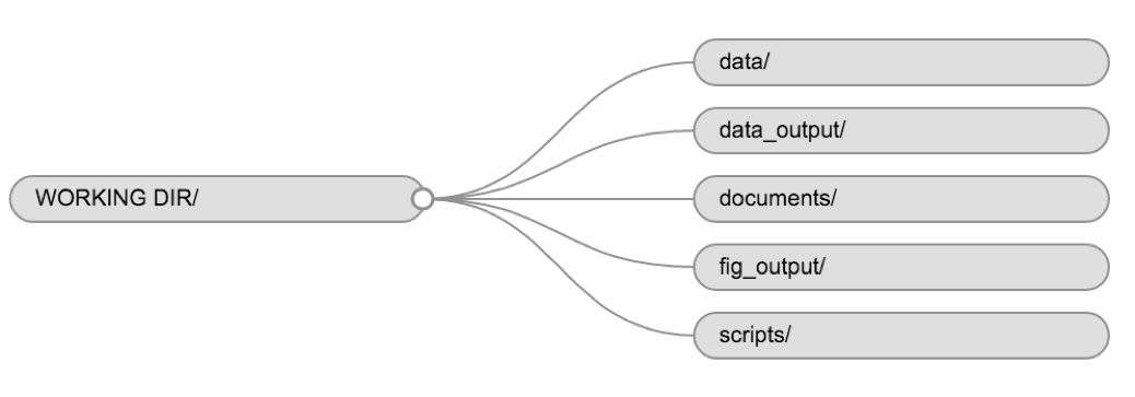
Using a consistent folder structure across your projects will help keep things organized and make it easy to find/file things in the future. This can be especially helpful when you have multiple projects. In general, you might create directories (folders) for scripts, data, and documents. Here are some examples of suggested directories:
-
data/Use this folder to store your raw data and intermediate datasets. For the sake of transparency and provenance, you should always keep a copy of your raw data accessible and do as much of your data cleanup and preprocessing programmatically (i.e., with scripts, rather than manually) as possible. -
data_output/When you need to modify your raw data, it might be useful to store the modified versions of the datasets in a different folder. -
documents/Used for outlines, drafts, and other text. -
fig_output/This folder can store the graphics that are generated by your scripts. -
scripts/A place to keep your R scripts for different analyses or plotting.
You may want additional directories or subdirectories depending on your project needs, but these should form the backbone of your working directory.
The working directory
The working directory is an important concept to understand. It is the place on your computer where R will look for and save files. When you write code for your project, your scripts should refer to files in relation to the root of your working directory and only to files within this structure.
Using RStudio projects makes this easy and ensures that your working
directory is set up properly. If you need to check it, you can use
getwd(). If for some reason your working directory is not
what it should be, you can change it in the RStudio interface by
navigating in the file browser to where your working directory should
be, then by clicking on the blue gear icon “More”, and selecting “Set As
Working Directory”. Alternatively, you can use
setwd("/path/to/working/directory") to reset your working
directory. However, your scripts should not include this line, because
it will fail on someone else’s computer.
Setting your working directory withsetwd()
Some points to note about setting your working directory:
The directory must be in quotation marks.
On Windows computers, directories in file paths are separated with a
backslash \. However, in R, you must use a forward slash
/. You can copy and paste from the Windows Explorer window
directly into R and use find/replace (Ctrl/Cmd + F) in R Studio to
replace all backslashes with forward slashes.
On Mac computers, open the Finder and navigate to the directory you
wish to set as your working directory. Right click on that folder and
press the options key on your keyboard. The ‘Copy “Folder
Name”’ option will transform into ’Copy “Folder Name” as Pathname. It
will copy the path to the folder to the clipboard. You can then paste
this into your setwd() function. You do not need to replace
backslashes with forward slashes.
After you set your working directory, you can use ./ to
represent it. So if you have a folder in your directory called
data, you can use read.csv(“./data”) to represent that
sub-directory.
Downloading the data and getting set up
Now that you have set your working directory, we will create our
folder structure using the dir.create() function.
For this lesson we will use the following folders in our working
directory: data/,
data_output/ and
fig_output/. Let’s write them all in
lowercase to be consistent. We can create them using the RStudio
interface by clicking on the “New Folder” button in the file pane
(bottom right), or directly from R by typing at console:
R
dir.create("data")
dir.create("data_output")
dir.create("fig_output")
Go to the Figshare page for this curriculum and download the dataset
called “books.csv”. The direct download link is: https://ndownloader.figshare.com/files/22031487.
Place this downloaded file in the data/ you just created.
Alternatively, you can do this directly from R by copying and
pasting this in your terminal (your instructor can place this chunk of
code in the Etherpad):
R
download.file("https://ndownloader.figshare.com/files/22031487",
              "data/books.csv", mode = "wb")
Now if you navigate to your data folder, the
books.csv file should be there. We now need to load it into
our R session.
tidyverse
R has some base functions for reading a local data file into your R
session–namely read.table() and read.csv(),
but these have some idiosyncrasies that were improved upon in the
readr package, which is installed and loaded with
tidyverse.
R
library(tidyverse) # loads the core tidyverse, including dplyr, readr, ggplot2, purrr
OUTPUT
── Attaching core tidyverse packages ──────────────────────── tidyverse 2.0.0 ──
✔ dplyr     1.1.2     ✔ purrr     1.0.1
✔ forcats   1.0.0     ✔ stringr   1.5.0
✔ ggplot2   3.4.2     ✔ tibble    3.2.1
✔ lubridate 1.9.2     ✔ tidyr     1.3.0
── Conflicts ────────────────────────────────────────── tidyverse_conflicts() ──
✖ dplyr::filter() masks stats::filter()
✖ dplyr::lag()    masks stats::lag()
ℹ Use the conflicted package (<http://conflicted.r-lib.org/>) to force all conflicts to become errors
To get our sample data into our R session, we will use the
read_csv() function and assign it to the books
value.
R
books <- read_csv("./data/books.csv")
You will see the message
Parsed with column specification, followed by each column
name and its data type. When you execute read_csv on a data
file, it looks through the first 1000 rows of each column and guesses
the data type for each column as it reads it into R. For example, in
this dataset, it reads SUBJECT as
col_character (character), and TOT.CHKOUT as
col_double. You have the option to specify the data type
for a column manually by using the col_types argument in
read_csv.
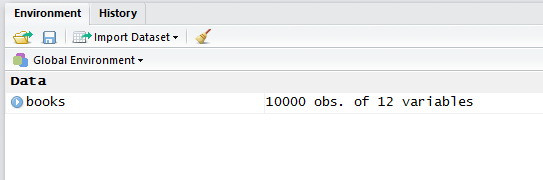
You should now have an R object called books in the
Environment pane: 10000 observations of 12 variables. We will be using
this data file in the next module.
Note
read_csv() assumes that fields are delineated by commas,
however, in several countries, the comma is used as a decimal separator
and the semicolon (;) is used as a field delineator. If you want to read
in this type of files in R, you can use the read_csv2
function. It behaves exactly like read_csv but uses
different parameters for the decimal and the field separators. If you
are working with another format, they can be both specified by the user.
Check out the help for read_csv() by typing
?read_csv to learn more. There is also the
read_tsv() for tab-separated data files, and
read_delim() allows you to specify more details about the
structure of your file.
What are data frames and tibbles?
Data frames are the de facto data structure for tabular data
in R, and what we use for data processing, statistics, and
plotting.
A data frame is the representation of data in the format of a table where the columns are vectors that all have the same length. Because columns are vectors, each column must contain a single type of data (e.g., characters, integers, factors). For example, here is a figure depicting a data frame comprising a numeric, a character, and a logical vector.

A data frame can be created by hand, but most commonly they are
generated by the functions read_csv() or
read_table(); in other words, when importing spreadsheets
from your hard drive (or the web).
A tibble is an extension of R data frames used by the
tidyverse. When the data is read using read_csv(),
it is stored in an object of class tbl_df,
tbl, and data.frame. You can see the class of
an object with class().
Inspecting data frames
When calling a tbl_df object (like books
here), there is already a lot of information about our data frame being
displayed such as the number of rows, the number of columns, the names
of the columns, and as we just saw the class of data stored in each
column. However, there are functions to extract this information from
data frames. Here is a non-exhaustive list of some of these functions.
Let’s try them out!
-
Size:
-
dim(books)- returns a vector with the number of rows in the first element, and the number of columns as the second element (the dimensions of the object) -
nrow(books)- returns the number of rows -
ncol(books)- returns the number of columns
-
-
Content:
-
head(books)- shows the first 6 rows -
tail(books)- shows the last 6 rows
-
-
Names:
-
names(books)- returns the column names (synonym ofcolnames()fordata.frameobjects)
-
-
Summary:
-
View(books)- look at the data in the viewer -
str(books)- structure of the object and information about the class, length and content of each column -
summary(books)- summary statistics for each column
-
Note: most of these functions are “generic”, they can be used on other types of objects besides data frames.
The map() function from purrr is a useful
way of running a function on all variables in a data frame or list. If
you loaded the tidyverse at the beginning of the session,
you also loaded purrr. Here we call class() on
books using map_chr(), which will return a
character vector of the classes for each variable.
R
map_chr(books, class)
OUTPUT
CALL...BIBLIO.        X245.ab         X245.c       LOCATION     TOT.CHKOUT
   "character"    "character"    "character"    "character"      "numeric"
      LOUTDATE        SUBJECT            ISN   CALL...ITEM.  X008.Date.One
   "character"    "character"    "character"    "character"    "character"
        BCODE2         BCODE1
   "character"    "character"
Indexing and subsetting data frames
Our books data frame has 2 dimensions: rows
(observations) and columns (variables). If we want to extract some
specific data from it, we need to specify the “coordinates” we want from
it. In the last session, we used square brackets [ ] to
subset values from vectors. Here we will do the same thing for data
frames, but we can now add a second dimension. Row numbers come first,
followed by column numbers. However, note that different ways of
specifying these coordinates lead to results with different classes.
R
## first element in the first column of the data frame (as a vector)
books[1, 1]
## first element in the 6th column (as a vector)
books[1, 6]
## first column of the data frame (as a vector)
books[[1]]
## first column of the data frame (as a data.frame)
books[1]
## first three elements in the 7th column (as a vector)
books[1:3, 7]
## the 3rd row of the data frame (as a data.frame)
books[3, ]
## equivalent to head_books <- head(books)
head_books <- books[1:6, ]
Dollar sign
The dollar sign $ is used to distinguish a specific
variable (column, in Excel-speak) in a data frame:
R
head(books$X245.ab) # print the first six book titles
OUTPUT
[1] "Bermuda Triangle /"
[2] "Invaders from outer space :|real-life stories of UFOs /"
[3] "Down Cut Shin Creek :|the pack horse librarians of Kentucky /"
[4] "The Chinese book of animal powers /"
[5] "Judge Judy Sheindlin's Win or lose by how you choose! /"
[6] "Judge Judy Sheindlin's You can't judge a book by its cover :|cool rules for school /"
R
# print the mean number of checkouts
mean(books$TOT.CHKOUT)
OUTPUT
[1] 2.2847
unique(), table(), and
duplicated()
Use unique() to see all the distinct values in a
variable:
R
unique(books$BCODE2)
OUTPUT
[1] "a" "w" "s" "m" "e" "4" "k" "5" "n" "o"Take that one step further with table() to get quick
frequency counts on a variable:
R
table(books$BCODE2) # frequency counts on a variable
OUTPUT
   4    5    a    e    k    m    n    o    s    w
   1    3 6983   68    3  109    2   21 1988  822
You can combine table() with relational operators:
R
table(books$TOT.CHKOUT > 50) # how many books have 50 or more checkouts?
OUTPUT
FALSE  TRUE
 9991     9
duplicated() will give you the a logical vector of
duplicated values.
R
duplicated(books$ISN)  # a TRUE/FALSE vector of duplicated values in the ISN column
!duplicated(books$ISN)  # you can put an exclamation mark before it to get non-duplicated values
table(duplicated(books$ISN))  # run a table of duplicated values
which(duplicated(books$ISN))  # get row numbers of duplicated values
Exploring missing values
You may also need to know the number of missing values:
R
sum(is.na(books)) # How many total missing values?
OUTPUT
[1] 14509R
colSums(is.na(books)) # Total missing values per column
OUTPUT
CALL...BIBLIO.        X245.ab         X245.c       LOCATION     TOT.CHKOUT
           561             12           2801              0              0
      LOUTDATE        SUBJECT            ISN   CALL...ITEM.  X008.Date.One
             0             63           2934           7980            158
        BCODE2         BCODE1
             0              0
R
table(is.na(books$ISN)) # use table() and is.na() in combination
OUTPUT
FALSE  TRUE
 7066  2934
R
booksNoNA <- na.omit(books) # Return only observations that have no missing values
Exercise
Call
View(books)to examine the data frame. Use the small arrow buttons in the variable name to sort tot_chkout by the highest checkouts. What item has the most checkouts?What is the class of the TOT.CHKOUT variable?
Use
table()andis.na()to find out how many NA values are in the ISN variable.Call
summary(books$TOT.CHKOUT). What can we infer when we compare the mean, median, and max?hist()will print a rudimentary histogram, which displays frequency counts. Callhist(books$TOT.CHKOUT). What is this telling us?
Highest checkouts:
Click, clack, moo : cows that type.class(books$TOT.CHKOUT)returnsnumerictable(is.na(books$ISN))returns 2934TRUEvaluesThe median is 0, indicating that, consistent with all book circulation I have seen, the majority of items have 0 checkouts.
As we saw in
summary(), the majority of items have a small number of checkouts
Logical tests
R contains a number of operators you can use to compare values. Use
help(Comparison) to read the R help file. Note that
two equal signs (==) are used for
evaluating equality (because one equals sign (=) is used
for assigning variables).
| operator | function |
|---|---|
< |
Less Than |
> |
Greater Than |
== |
Equal To |
<= |
Less Than or Equal To |
>= |
Greater Than or Equal To |
!= |
Not Equal To |
%in% |
Has a Match In |
is.na() |
Is NA |
!is.na() |
Is Not NA |
Sometimes you need to do multiple logical tests (think Boolean
logic). Use help(Logic) to read the help file.
| operator | function |
|---|---|
& |
boolean AND |
| ` | ` |
! |
Boolean NOT |
any() |
Are some values true? |
all() |
Are all values true? |
Content from Data cleaning & transformation with dplyr
Last updated on 2024-03-12 | Edit this page
Overview
Questions
- How can I select specific rows and/or columns from a data frame?
- How can I combine multiple commands into a single command?
- How can create new columns or remove existing columns from a data frame?
- How can I reformat a dataframe to meet my needs?
Objectives
- Describe the purpose of an R package and the
dplyrandtidyrpackages. - Select certain columns in a data frame with the
dplyrfunctionselect. - Select certain rows in a data frame according to filtering
conditions with the
dplyrfunctionfilter. - Link the output of one
dplyrfunction to the input of another function with the ‘pipe’ operator%>%. - Add new columns to a data frame that are functions of existing
columns with
mutate. - Use the split-apply-combine concept for data analysis.
- Use
summarize,group_by, andcountto split a data frame into groups of observations, apply a summary statistics for each group, and then combine the results. - Describe the concept of a wide and a long table format and for which purpose those formats are useful.
- Describe what key-value pairs are.
- Reshape a data frame from long to wide format and back with the
pivot_widerandpivot_longercommands from thetidyrpackage. - Export a data frame to a csv file.
Getting set up
Open your R Project file
If you have not already done so, open your R Project file
(library_carpentry.Rproj) created in the
Before We Start lesson.
If you did not complete that step then do the following:
- Under the
Filemenu, click onNew project, chooseNew directory, thenNew project - Enter the name
library_carpentryfor this new folder (or “directory”). This will be your working directory for the rest of the day. - Click on
Create project - Create a new file where we will type our scripts. Go to File >
New File > R script. Click the save icon on your toolbar and save
your script as “
script.R”. - Copy and paste the below lines of code to create three new subdirectories and download the data:
R
library(fs)   # https://fs.r-lib.org/.  fs is a cross-platform, uniform interface to file system operations via R.
dir_create("data")
dir_create("data_output")
dir_create("fig_output")
download.file("https://ndownloader.figshare.com/files/22031487",
              "data/books.csv", mode = "wb")
Load the tidyverse and data frame into your R
session
Load the tidyverse
R
library(tidyverse)
OUTPUT
── Attaching core tidyverse packages ──────────────────────── tidyverse 2.0.0 ──
✔ dplyr     1.1.2     ✔ purrr     1.0.1
✔ forcats   1.0.0     ✔ stringr   1.5.0
✔ ggplot2   3.4.2     ✔ tibble    3.2.1
✔ lubridate 1.9.2     ✔ tidyr     1.3.0
── Conflicts ────────────────────────────────────────── tidyverse_conflicts() ──
✖ dplyr::filter() masks stats::filter()
✖ dplyr::lag()    masks stats::lag()
ℹ Use the conflicted package (<http://conflicted.r-lib.org/>) to force all conflicts to become errors
And the books data we saved in the previous lesson.
R
books <- read_csv("data/books.csv") # load the data and assign it to books
Transforming data with dplyr
We are now entering the data cleaning and transforming phase. While
it is possible to do much of the following using Base R functions (in
other words, without loading an external package) dplyr
makes it much easier. Like many of the most useful R packages,
dplyr was developed by data scientist http://hadley.nz/.
dplyr is a package for making tabular data manipulation
easier by using a limited set of functions that can be combined to
extract and summarize insights from your data. It pairs nicely with
tidyr which enables you to swiftly convert
between different data formats (long vs. wide) for plotting and
analysis.
dplyr is also part of the tidyverse. Let’s
make sure we are all on the same page by loading the
tidyverse and the books dataset we downloaded
earlier.
We’re going to learn some of the most common
dplyr functions:
-
rename(): rename columns -
recode(): recode values in a column -
select(): subset columns -
filter(): subset rows on conditions -
mutate(): create new columns by using information from other columns -
group_by()andsummarize(): create summary statistics on grouped data -
arrange(): sort results -
count(): count discrete values
Renaming variables
It is often necessary to rename variables to make them more
meaningful. If you print the names of the sample books
dataset you can see that some of the vector names are not particularly
helpful:
R
glimpse(books) # print names of the books data frame to the console
OUTPUT
Rows: 10,000
Columns: 12
$ CALL...BIBLIO. <chr> "001.94 Don 2000", "001.942 Bro 1999", "027.073 App 200…
$ X245.ab        <chr> "Bermuda Triangle /", "Invaders from outer space :|real…
$ X245.c         <chr> "written by Andrew Donkin.", "written by Philip Brooks.…
$ LOCATION       <chr> "juv", "juv", "juv", "juv", "juv", "juv", "juv", "juv",…
$ TOT.CHKOUT     <dbl> 6, 2, 3, 6, 7, 6, 4, 2, 4, 13, 6, 7, 3, 22, 2, 9, 4, 8,…
$ LOUTDATE       <chr> "11-21-2013 9:44", "02-07-2004 15:29", "10-16-2007 10:5…
$ SUBJECT        <chr> "Readers (Elementary)|Bermuda Triangle -- Juvenile lite…
$ ISN            <chr> "0789454165 (hbk.)~0789454157 (pbk.)", "0789439999 (har…
$ CALL...ITEM.   <chr> "001.94 Don 2000", "001.942 Bro 1999", "027.073 App 200…
$ X008.Date.One  <chr> "2000", "1999", "2001", "1999", "2000", "2001", "2001",…
$ BCODE2         <chr> "a", "a", "a", "a", "a", "a", "a", "a", "a", "a", "a", …
$ BCODE1         <chr> "j", "j", "j", "j", "j", "j", "j", "j", "j", "j", "j", …
There are many ways to rename variables in R, but the
rename() function in the dplyr package is the
easiest and most straightforward. The new variable name comes first. See
help(rename).
Here we rename the X245.ab variable. Make sure you assign the output
to your books value, otherwise it will just print it to the
console. In other words, we are overwriting the previous
books value with the new one, with X245.ab
renamed to title.
R
# rename the . Make sure you return (<-) the output to your
# variable, otherwise it will just print it to the console
books <- rename(books,
                title = X245.ab)
R
# rename multiple variables at once
books <- rename(books,
                author = X245.c,
                callnumber = CALL...BIBLIO.,
                isbn = ISN,
                pubyear = X008.Date.One,
                subCollection = BCODE1,
                format = BCODE2,
                location = LOCATION,
                tot_chkout = TOT.CHKOUT,
                loutdate = LOUTDATE,
                subject = SUBJECT)
books
OUTPUT
# A tibble: 10,000 × 12
   callnumber        title     author location tot_chkout loutdate subject isbn
   <chr>             <chr>     <chr>  <chr>         <dbl> <chr>    <chr>   <chr>
 1 001.94 Don 2000   Bermuda … writt… juv               6 11-21-2… Reader… 0789…
 2 001.942 Bro 1999  Invaders… writt… juv               2 02-07-2… Reader… 0789…
 3 027.073 App 2001  Down Cut… by Ka… juv               3 10-16-2… Packho… 0060…
 4 133.5 Hua 1999    The Chin… by Ch… juv               6 11-22-2… Astrol… 0060…
 5 170 She 2000      Judge Ju… illus… juv               7 04-10-2… Childr… 0060…
 6 170.44 She 2001   Judge Ju… illus… juv               6 11-12-2… Conduc… 0060…
 7 220.9505 Gil 2001 A young … retol… juv               4 12-01-2… Bible … 0060…
 8 225.9505 McC 1999 God's Ki… retol… juv               2 08-06-2… Bible … 0689…
 9 292.13 McC 2001   Roman my… retol… juv               4 04-03-2… Mythol… 0689…
10 292.211 McC 1998  Greek go… retol… juv              13 11-16-2… Gods, … 0689…
# ℹ 9,990 more rows
# ℹ 4 more variables: CALL...ITEM. <chr>, pubyear <chr>, format <chr>,
# subCollection <chr>R
books <- rename(books,
                callnumber2 = CALL...ITEM.)
Recoding values
It is often necessary to recode or reclassify values in your data.
For example, in the sample dataset provided to you, the
sub_collection (formerly BCODE1) and
format (formerly BCODE2) variables contain
single characters.
You can do this easily using the recode() function, also
in the dplyr package. Unlike rename(), the old
value comes first here. Also notice that we are overwriting the
books$subCollection variable.
R
# first print to the console all of the unique values you will need to recode
distinct(books, subCollection)
OUTPUT
FALSE # A tibble: 10 × 1
FALSE    subCollection
FALSE    <chr>
FALSE  1 j
FALSE  2 b
FALSE  3 u
FALSE  4 r
FALSE  5 -
FALSE  6 s
FALSE  7 c
FALSE  8 z
FALSE  9 a
FALSE 10 t
R
books$subCollection <- recode(books$subCollection,
                                      "-" = "general collection",
                                      u = "government documents",
                                      r = "reference",
                                      b = "k-12 materials",
                                      j = "juvenile",
                                      s = "special collections",
                                      c = "computer files",
                                      t = "theses",
                                      a = "archives",
                                      z = "reserves")
books
OUTPUT
FALSE # A tibble: 10,000 × 12
FALSE    callnumber        title     author location tot_chkout loutdate subject isbn
FALSE    <chr>             <chr>     <chr>  <chr>         <dbl> <chr>    <chr>   <chr>
FALSE  1 001.94 Don 2000   Bermuda … writt… juv               6 11-21-2… Reader… 0789…
FALSE  2 001.942 Bro 1999  Invaders… writt… juv               2 02-07-2… Reader… 0789…
FALSE  3 027.073 App 2001  Down Cut… by Ka… juv               3 10-16-2… Packho… 0060…
FALSE  4 133.5 Hua 1999    The Chin… by Ch… juv               6 11-22-2… Astrol… 0060…
FALSE  5 170 She 2000      Judge Ju… illus… juv               7 04-10-2… Childr… 0060…
FALSE  6 170.44 She 2001   Judge Ju… illus… juv               6 11-12-2… Conduc… 0060…
FALSE  7 220.9505 Gil 2001 A young … retol… juv               4 12-01-2… Bible … 0060…
FALSE  8 225.9505 McC 1999 God's Ki… retol… juv               2 08-06-2… Bible … 0689…
FALSE  9 292.13 McC 2001   Roman my… retol… juv               4 04-03-2… Mythol… 0689…
FALSE 10 292.211 McC 1998  Greek go… retol… juv              13 11-16-2… Gods, … 0689…
FALSE # ℹ 9,990 more rows
FALSE # ℹ 4 more variables: callnumber2 <chr>, pubyear <chr>, format <chr>,
FALSE #   subCollection <chr>
Do the same for the format column. Note that you must
put "5" and "4" into quotation marks for the
function to operate correctly.
R
books$format <- recode(books$format,
                              a = "book",
                              e = "serial",
                              w = "microform",
                              s = "e-gov doc",
                              o = "map",
                              n = "database",
                              k = "cd-rom",
                              m = "image",
                              "5" = "kit/object",
                              "4" = "online video")
Subsetting dataframes
Subsetting using filter() in the dplyr
package
In the last lesson we learned how to subset a data frame using
brackets. As with other R functions, the dplyr package
makes it much more straightforward, using the filter()
function.
Here we will create a subset of books called
booksOnly, which includes only those items where the format
is books. Notice that we use two equal signs == as the
logical operator:
R
booksOnly <- filter(books, format == "book") # filter books to return only those items where the format is books
You can also use multiple filter conditions. Here, the order matters: first we filter to include only books, then of the results, we include only items that have more than zero checkouts.
R
bookCheckouts <- filter(books,
                        format == "book",
                        tot_chkout > 0)
How many items were removed? You can find out functionally with:
R
nrow(books) - nrow(bookCheckouts)
OUTPUT
FALSE [1] 5733You can then check the summary statistics of checkouts for books with more than zero checkouts. Notice how different these numbers are from the previous lesson, when we kept zero in. The median is now 3 and the mean is 5.
R
summary(bookCheckouts$tot_chkout)
OUTPUT
FALSE    Min. 1st Qu.  Median    Mean 3rd Qu.    Max.
FALSE   1.000   2.000   3.000   5.281   6.000 113.000
If you want to filter on multiple conditions within the same
variable, use the %in% operator combined with a vector of
all the values you wish to include within c(). For example,
you may want to include only items in the format serial and
microform:
R
serial_microform <- filter(books, format %in% c("serial", "microform"))
R
booksJuv <- filter(books,
               format == "book",
               subCollection ==  "juvenile")
mean(booksJuv$tot_chkout)
OUTPUT
[1] 10.41404Selecting variables
The select() function allows you to keep or remove
specific columns It also provides a convenient way to reorder
variables.
R
# specify the variables you want to keep by name
booksTitleCheckouts <- select(books, title, tot_chkout)
booksTitleCheckouts
OUTPUT
# A tibble: 10,000 × 2
   title                                                              tot_chkout
   <chr>                                                                   <dbl>
 1 Bermuda Triangle /                                                          6
 2 Invaders from outer space :|real-life stories of UFOs /                     2
 3 Down Cut Shin Creek :|the pack horse librarians of Kentucky /               3
 4 The Chinese book of animal powers /                                         6
 5 Judge Judy Sheindlin's Win or lose by how you choose! /                     7
 6 Judge Judy Sheindlin's You can't judge a book by its cover :|cool…          6
 7 A young child's Bible /                                                     4
 8 God's Kingdom :|stories from the New Testament /                            2
 9 Roman myths /                                                               4
10 Greek gods and goddesses /                                                 13
# ℹ 9,990 more rows
R
# specify the variables you want to remove with a -
books <- select(books, -location)

# reorder columns, combined with everything()
booksReordered <- select(books, title, tot_chkout, loutdate, everything())
Ordering data
The arrange() function in the dplyr package
allows you to sort your data by alphabetical or numerical order.
R
booksTitleArrange <- arrange(books, title)

# use desc() to sort a variable in descending order
booksHighestChkout <- arrange(books, desc(tot_chkout))
booksHighestChkout
OUTPUT
# A tibble: 10,000 × 11
   callnumber title author tot_chkout loutdate subject isbn  callnumber2 pubyear
   <chr>      <chr> <chr>       <dbl> <chr>    <chr>   <chr> <chr>       <chr>
 1 E Cro 2000 Clic… by Do…        113 01-23-2… Cows -… 0689… E Cro 2000  2000
 2 PZ7.W6367… The … by Da…        106 03-07-2… Pigs -… 0618… 398.2452 W… 2001
 3 <NA>       Cook… Janet…        103 03-13-2… Cake -… 0152… E Ste 1999  1999
 4 PZ7.D5455… Beca… Kate …         79 03-27-2… Dogs -… 0763… Fic Dic 20… 2000
 5 PZ7.C6775… Upto… Bryan…         69 02-05-2… Harlem… 9780… E Col 2000  2000
 6 <NA>       <NA>  <NA>           64 08-23-2… <NA>    <NA>  #1  ENC. C… <NA>
 7 F379.N59 … Thro… Ruby …         63 11-01-2… Bridge… 0590… 920 Bri 19… 1999
 8 PZ7.C9413… Bud,… Chris…         63 04-03-2… Runawa… 0385… Fic Cur 19… 1999
 9 E Mar 1992 Brow… by Bi…         61 02-16-2… Color … 0805… E Mar 1992  1992
10 PZ7.P338 … A ye… Richa…         47 03-26-2… Grandm… 0803… Fic Pec 20… 2000
# ℹ 9,990 more rows
# ℹ 2 more variables: format <chr>, subCollection <chr>
R
# order data based on multiple variables (e.g. sort first by checkout, then by publication year)
booksChkoutYear <- arrange(books, desc(tot_chkout), desc(pubyear))
Creating new variables
The mutate() function allows you to create new
variables. Here, we use the str_sub() function from the
stringr package to extract the first character of the
callnumber variable (the call number class) and put it into
a new column called call_class.
R
booksLC <- mutate(books,
                  call_class = str_sub(callnumber, 1, 1))
There are two numbers because you must specify a start and an end value–here, we start with the first character, and end with the first character.
mutate() is also helpful to coerce a column from one
data type to another. For example, we can see there are some errors in
the pubyear variable–some dates are 19zz or
uuuu. As a result, this variable was read in as a
character rather than an integer.
R
books <- mutate(books, pubyear = as.integer(pubyear))
WARNING
Warning: There was 1 warning in `mutate()`.
ℹ In argument: `pubyear = as.integer(pubyear)`.
Caused by warning:
! NAs introduced by coercion
We see the error message NAs introduced by coercion.
This is because non-numerical variables become NA and the
remainder become integers.
Putting it all together with %>%
The Pipe
Operator %>% is loaded with the
tidyverse. It takes the output of one statement and makes
it the input of the next statement. You can think of it as “then” in
natural language. So instead of making a bunch of intermediate data
frames and cluttering up your workspace, you can run multiple functions
at once. You can type the pipe with Ctrl + Shift +
M if you have a PC or Cmd + Shift +
M if you have a Mac.
So in the following example, the books tibble is first
called, then the format is filtered to include only
book, then only the title and
tot_chkout columns are selected, and finally the data is
rearranged from most to least checkouts.
R
myBooks <- books %>%
  filter(format == "book") %>%
  select(title, tot_chkout) %>%
  arrange(desc(tot_chkout))
myBooks
OUTPUT
# A tibble: 6,983 × 2
   title                                      tot_chkout
   <chr>                                           <dbl>
 1 Click, clack, moo :|cows that type /              113
 2 The three pigs /                                  106
 3 Cook-a-doodle-doo! /                              103
 4 Because of Winn-Dixie /                            79
 5 Uptown /                                           69
 6 Through my eyes /                                  63
 7 Bud, not Buddy /                                   63
 8 Brown bear, brown bear, what do you see? /         61
 9 A year down yonder /                               47
10 Wemberly worried /                                 43
# ℹ 6,973 more rows
Playing with pipes%>%
- Create a new data frame
booksKidswith these conditions:
-
filter()to includesubCollectionjuvenile & k-12 materials andformatbooks. -
select()only title, call number, total checkouts, and publication year -
arrange()by total checkouts in descending order
- Use
mean()to check the average number of checkouts for thebooksKidsdata frame.
R
booksKids <- books %>%
  filter(subCollection %in% c("juvenile", "k-12 materials"),
  format == "book") %>%
select(title, callnumber, tot_chkout, pubyear) %>%
arrange(desc(tot_chkout))
mean(booksKids$tot_chkout)
OUTPUT
[1] 9.336331Split-apply-combine data analysis and the summarize()
function
Many data analysis tasks can be approached using the
split-apply-combine paradigm: split the data into groups, apply
some analysis to each group, and then combine the results.
dplyr makes this very easy through the use
of the group_by() function.
The summarize() function
group_by() is often used together with
summarize(), which collapses each group into a single-row
summary of that group. group_by() takes as arguments the
column names that contain the categorical variables for
which you want to calculate the summary statistics.
So to compute the average checkouts by format:
R
books %>%
  group_by(format) %>%
  summarize(mean_checkouts = mean(tot_chkout))
OUTPUT
# A tibble: 10 × 2
   format       mean_checkouts
   <chr>                 <dbl>
 1 book                3.23
 2 cd-rom              0.333
 3 database            0
 4 e-gov doc           0.0402
 5 image               0.0275
 6 kit/object          1.33
 7 map                10.6
 8 microform           0.00122
 9 online video        0
10 serial              0
Books and maps have the highest, and as we would expect, databases, online videos, and serials have zero checkouts.
Here is a more complex example:
R
books %>%
  filter(format == "book") %>%
  mutate(call_class = str_sub(callnumber, 1, 1)) %>%
  group_by(call_class) %>%
  summarize(count = n(),
            sum_tot_chkout = sum(tot_chkout)) %>%
  arrange(desc(sum_tot_chkout))
OUTPUT
# A tibble: 34 × 3
   call_class count sum_tot_chkout
   <chr>      <int>          <dbl>
 1 E            487           3114
 2 <NA>         459           3024
 3 H           1142           2902
 4 P            800           2645
 5 F            240           1306
 6 Q            333           1305
 7 B            426           1233
 8 R            193            981
 9 L            358            862
10 5             60            838
# ℹ 24 more rows
Let’s break this down step by step:
- First we call the
booksdata frame - We then pipe through
filter()to include only books - We then create a new column with
mutate()calledcall_classby using thestr_sub()function to keep the first character of thecall_numbervariable - We then
group_by()our newly createdcall_classvariable - We then create two summary columns by using
summarize()- take the number
n()of items percall_classand assign it to a column calledcount - take the the
sum()oftot_chkoutpercall_classand assign the result to a column calledsum_tot_chkout
- take the number
- Finally, we arrange
sum_tot_chkoutin descending order, so we can see the class with the most total checkouts. We can see it is theEclass (History of America), followed byNA(items with no call number data), followed byH(Social Sciences) andP(Language and Literature).
Pattern matching
Cleaning text with the stringr package is easier when
you have a basic understanding of ‘regex’, or regular expression pattern
matching. Regex is especially useful for manipulating strings
(alphanumeric data), and is the backbone of search-and-replace
operations in most applications. Pattern matching is common to all
programming languages but regex syntax is often code-language specific.
Below, find an example of using pattern matching to find and replace
data in R:
- Remove the trailing slash in the title column
- Modify the punctuation separating the title from a subtitle
Note: If the final product of this data will be imported into an ILS, you may not want to alter the MARC specific punctuation. All other audiences will appreciate the text normalizing steps.
Read more about matching patterns with regular expressions.
R
books %>%
  mutate(title_modified = str_remove(title, "/$")) %>%     # remove the trailing slash
  mutate(title_modified = str_replace(title_modified, "\\s:\\|", ": ")) %>%   # replace ' :|' with ': '
  select(title_modified, title)
OUTPUT
# A tibble: 10,000 × 2
   title_modified                                                          title
   <chr>                                                                   <chr>
 1 "Bermuda Triangle "                                                     Berm…
 2 "Invaders from outer space: real-life stories of UFOs "                 Inva…
 3 "Down Cut Shin Creek: the pack horse librarians of Kentucky "           Down…
 4 "The Chinese book of animal powers "                                    The …
 5 "Judge Judy Sheindlin's Win or lose by how you choose! "                Judg…
 6 "Judge Judy Sheindlin's You can't judge a book by its cover: cool rule… Judg…
 7 "A young child's Bible "                                                A yo…
 8 "God's Kingdom: stories from the New Testament "                        God'…
 9 "Roman myths "                                                          Roma…
10 "Greek gods and goddesses "                                             Gree…
# ℹ 9,990 more rows
Exporting data
Now that you have learned how to use
dplyr to extract information from or
summarize your raw data, you may want to export these new data sets to
share them with your collaborators or for archival.
Similar to the read_csv() function used for reading CSV
files into R, there is a write_csv() function that
generates CSV files from data frames.
Before using write_csv(), we are going to create a new
folder, data_output, in our working directory that will
store this generated dataset. We don’t want to write generated datasets
in the same directory as our raw data. It’s good practice to keep them
separate. The data folder should only contain the raw,
unaltered data, and should be left alone to make sure we don’t delete or
modify it. In contrast, our script will generate the contents of the
data_output directory, so even if the files it contains are
deleted, we can always re-generate them.
In preparation for our next lesson on plotting, we are going to create a version of the dataset with most of the changes we made above. We will first read in the original, then make all the changes with pipes.
R
books_reformatted <- read_csv("./data/books.csv") %>%
  rename(title = X245.ab,
         author = X245.c,
         callnumber = CALL...BIBLIO.,
         isbn = ISN,
         pubyear = X008.Date.One,
         subCollection = BCODE1,
         format = BCODE2,
         location = LOCATION,
         tot_chkout = TOT.CHKOUT,
         loutdate = LOUTDATE,
         subject = SUBJECT,
         callnumber2 = CALL...ITEM.) %>%
  mutate(pubyear = as.integer(pubyear),
         call_class = str_sub(callnumber, 1, 1),
         subCollection = recode(subCollection,
                                "-" = "general collection",
                                u = "government documents",
                                r = "reference",
                                b = "k-12 materials",
                                j = "juvenile",
                                s = "special collections",
                                c = "computer files",
                                t = "theses",
                                a = "archives",
                                z = "reserves"),
         format = recode(format,
                         a = "book",
                         e = "serial",
                         w = "microform",
                         s = "e-gov doc",
                         o = "map",
                         n = "database",
                         k = "cd-rom",
                         m = "image",
                         "5" = "kit/object",
                         "4" = "online video"))
This chunk of code read the CSV, renamed the variables, used
mutate() in combination with recode() to
recode the format and subCollection values,
used mutate() in combination with as.integer()
to coerce pubyear to integer, and used
mutate() in combination with str_sub to create
the new varable call_class.
We now write it to a CSV and put it in the data/output
sub-directory:
R
write_csv(books_reformatted, "./data_output/books_reformatted.csv")
Help with dplyr
- Read more about
dplyrat https://dplyr.tidyverse.org/. - In your console, after loading
library(dplyr), runvignette("dplyr")to read an extremely helpful explanation of how to use it. - See the http://r4ds.had.co.nz/transform.html in Garrett Grolemund and Hadley Wickham’s book R for Data Science.
- Watch this Data School video: https://www.youtube.com/watch?v=jWjqLW-u3hc
Wrangling dataframes with tidyr
Content from Data Visualisation with ggplot2
Last updated on 2024-03-12 | Edit this page
Overview
Questions
- What are the components of a ggplot?
- How do I create scatterplots, boxplots, and barplots?
- How can I change the aesthetics (ex. colour, transparency) of my plot?
- How can I create multiple plots at once?
Objectives
- Produce scatter plots, boxplots, and time series plots using ggplot.
- Set universal plot settings.
- Describe what faceting is and apply faceting in ggplot.
- Modify the aesthetics of an existing ggplot plot (including axis labels and color).
- Build complex and customized plots from data in a data frame.
Getting set up
Set up your directories and data
If you have not already done so, open your R Project file
(library_carpentry.Rproj) created in the
Before We Start lesson.
If you did not complete that step then do the following. Only do this if you didn’t complete it in previous lessons.
- Under the
Filemenu, click onNew project, chooseNew directory, thenNew project - Enter the name
library_carpentryfor this new folder (or “directory”). This will be your working directory for the rest of the day. - Click on
Create project - Create a new file where we will type our scripts. Go to File >
New File > R script. Click the save icon on your toolbar and save
your script as “
script.R”. - Copy and paste the below lines of code to create three new
subdirectories and download the original and the reformatted
booksdata:
R
library(fs)   # https://fs.r-lib.org/.  fs is a cross-platform, uniform interface to file system operations via R.
dir_create("data")
dir_create("data_output")
dir_create("fig_output")
download.file("https://ndownloader.figshare.com/files/22031487",
              "data/books.csv", mode = "wb")
download.file("https://ndownloader.figshare.com/files/22051506",
              "data_output/books_reformatted.csv", mode = "wb")
Load the tidyverse and data frame into your R
session
Load the tidyverse and the lubridate
packages. lubridate is installed with the tidyverse, but is
not one of the core tidyverse packages loaded with
library(tidyverse), so it needs to be explicitly called.
lubridate makes working with dates and times easier in
R.
R
library(tidyverse) # load the core tidyverse
OUTPUT
── Attaching core tidyverse packages ──────────────────────── tidyverse 2.0.0 ──
✔ dplyr     1.1.2     ✔ purrr     1.0.1
✔ forcats   1.0.0     ✔ stringr   1.5.0
✔ ggplot2   3.4.2     ✔ tibble    3.2.1
✔ lubridate 1.9.2     ✔ tidyr     1.3.0
── Conflicts ────────────────────────────────────────── tidyverse_conflicts() ──
✖ dplyr::filter() masks stats::filter()
✖ dplyr::lag()    masks stats::lag()
ℹ Use the conflicted package (<http://conflicted.r-lib.org/>) to force all conflicts to become errors
R
library(lubridate) # load lubridate
We also load the books_reformatted data we saved in the
previous lesson. We’ll assign it to books2.
R
books2 <- read_csv("data_output/books_reformatted.csv") # load the data and assign it to books
Plotting with ggplot2
Base R contains a number of functions for quick data visualization
such as plot() for scatter plots, barplot(),
hist() for histograms, and boxplot(). However,
just as data manipulation is easier with dplyr than Base R,
so data visualization is easier with ggplot2 than Base R.
ggplot2 is a “grammar” for
data visualization also created by Hadley Wickham, as an
implementation of Leland Wilkinson’s Grammar of
Graphics.
ggplot is a plotting package that makes it simple to
create complex plots from data stored in a data frame. It provides a
programmatic interface for specifying what variables to plot, how they
are displayed, and general visual properties. Therefore, we only need
minimal changes if the underlying data change or if we decide to change
from a bar plot to a scatterplot. This helps in creating publication
quality plots with minimal amounts of adjustments and tweaking.
ggplot2 functions like data in the ‘long’ format, i.e.,
a column for every dimension, and a row for every observation.
Well-structured data will save you lots of time when making figures with
ggplot2
ggplot graphics are built step by step by adding new elements. Adding layers in this fashion allows for extensive flexibility and customization of plots.
To build a ggplot, we will use the following basic template that can be used for different types of plots:
ggplot(data = <DATA>, mapping = aes(<MAPPINGS>)) + <GEOM_FUNCTION>()- use the
ggplot()function and bind the plot to a specific data frame using thedataargument
When you run the ggplot() function, it plots directly to
the Plots tab in the Navigation Pane (lower right). Alternatively, you
can assign a plot to an R object, then call print()to view
the plot in the Navigation Pane.
Let’s create a booksPlot and limit our visualization to
only items in subCollection general collection, juvenile,
and k-12, and filter out items with NA in
call_class. We do this by using the | key on the
keyboard to specify a boolean OR, and use the !is.na()
function to keep only those items that are NOT NA in the
call_class column.
R
# create a new data frame
booksPlot <- books2 %>%
  filter(subCollection == "general collection" |
           subCollection == "juvenile" |
           subCollection == "k-12 materials",
         !is.na(call_class))
ggplot2
ggplot2 functions like data in the ‘long’
format, i.e., a column for every dimension, and a row for every
observation. Well-structured data will save you lots of time when making
figures with ggplot2
ggplot graphics are built step by step by adding new elements. Adding layers in this fashion allows for extensive flexibility and customization of plots.
To build a ggplot, we will use the following basic template that can be used for different types of plots:
ggplot(data = <DATA>, mapping = aes(<MAPPINGS>)) + <GEOM_FUNCTION>()Use the ggplot() function and bind the plot to a
specific data frame using the data argument.
R
ggplot(data = booksPlot) # a blank canvas

Not very interesting. We need to add layers to it by defining a
mapping aesthetic and adding geoms.
Define a mapping with aes() and display data with
geoms
Define a mapping (using the aesthetic (aes()) function),
by selecting the variables to be plotted and specifying how to present
them in the graph, e.g. as x/y positions or characteristics such as
size, shape, color, etc.
R
ggplot(data = booksPlot, mapping = aes(x = call_class)) # define the x axis aesthetic
Here we define the x axes, but because we have not yet added any
geoms, we still do not see any data being visualized.
Data is visualized in the canvas with “geometric shapes” such as bars
and lines; what are called geoms. In your console, type
geom_ and press the tab key to see the geoms included–there
are over 30. For example:
-
geom_point()for scatter plots, dot plots, etc. -
geom_boxplot()for boxplots -
geom_bar()for barplots -
geom_line()for trend lines, time series, etc.
Each geom takes a mapping argument within the
aes() call. This is called the aesthetic mapping
argument. In other words, inside the geom function is an
aes() function, and inside aes() is a mapping
argument specifying how to map the variables inside the visualization.
ggplot then looks for that variable inside the data argument, and plots
it accordingly.
For example, in the below expression, the call_class
variable is being mapped to the x axis in the geometric
shape of a bar. In this example, the y axis (count) is not specified,
nor is it a variable in the original dataset, but is the result of
geom_bar() binning your data inside each call number class and
plotting the bin counts (the number of items falling into each bin).
To add a geom to the plot use the + operator.
R
# add a bar geom and set call_class as the x axis
ggplot(data = booksPlot, mapping = aes(x = call_class)) +
  geom_bar()
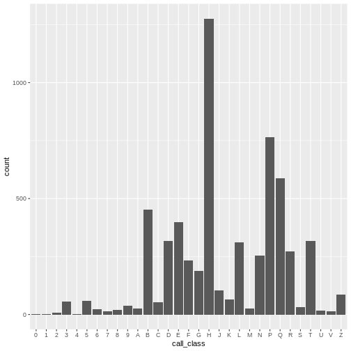
We can see that there are about 1,500 books in the H class, 1,000 books in the P class, 700 books in the E class, etc. As we shall see, the number of E and F books are deceptively large, as easy books and fiction books both begin with E and are thus lumped into that category, though they are not of the E and F Library of Congress call number classification.
ggplottips
- Anything you put in the
ggplot()function can be seen by any geom layers that you add (i.e., these are universal plot settings). This includes the x- and y-axis mapping you set up inaes(). - You can also specify mappings for a given geom independently of the
mapping defined globally in the
ggplot()function. - The
+sign used to add new layers must be placed at the end of the line containing the previous layer. If, instead, the+sign is added at the beginning of the line containing the new layer,ggplot2will not add the new layer and will return an error message.
Univariate geoms
“Univariate” refers to a single variable. A histogram is a
univariate plot: it shows the frequency counts of each value inside a
single variable. Let’s say we want to visualize a frequency distibution
of checkouts in the booksPlot data. In other words, how
many items have 1 checkout? How many have 2 checkouts? And so on.
R
ggplot(data = booksPlot, mapping = aes(x = tot_chkout)) +
  geom_histogram()
OUTPUT
`stat_bin()` using `bins = 30`. Pick better value with `binwidth`.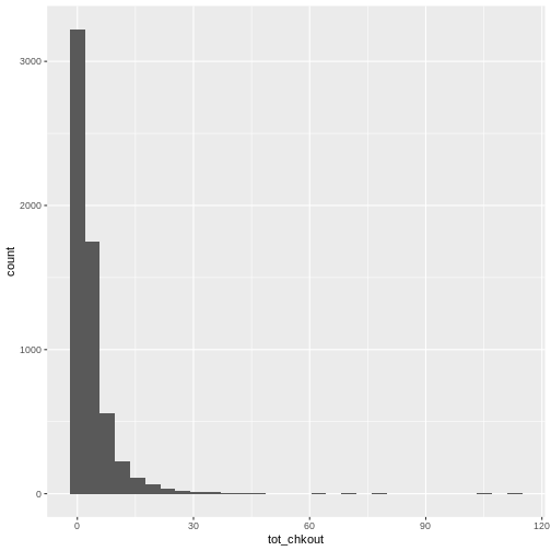
As we have seen in previous lessons, the overwhelming majority of books have a small amount of usage, so the plot is heavily skewed. As anyone who has done collection analysis has encountered, this is a very common issue. It can be addressed in two ways:
First, add a binwidth argument to aes(). In
a histogram, each bin contains the number of occurrences of items in the
data set that are contained within that bin. As stated in the
documentation for ?geom_histogram, “You should always
override this value, exploring multiple widths to find the best to
illustrate the stories in your data.”
Second, change the scales of the y axes by adding
another argument to ggplot:
R
ggplot(data = booksPlot) +
  geom_histogram(aes(x = tot_chkout), binwidth = 10) +
  scale_y_log10()
WARNING
Warning: Transformation introduced infinite values in continuous y-axisWARNING
Warning: Removed 2 rows containing missing values (`geom_bar()`).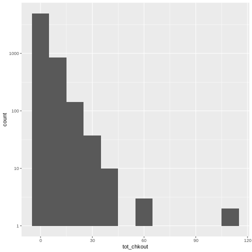
Notice the scale y axis now goes from 0-10, 10-100, 100-1000, and 1000-10000. This is called “logarithmic scale” and is based on orders of magnitude. We can therefore see that over 5,000 books (on the y axis) have between 0-10 checkouts (on the x axis), 1,000 books have 10-20 checkouts, and further down on the x axis, a handful of books have 60-70 checkouts, and a handful more have around 100 checkouts.
We can check this with table():
R
table(booksPlot$tot_chkout)
OUTPUT
   0    1    2    3    4    5    6    7    8    9   10   11   12   13   14   15
2348  875  638  464  362  282  199  146  118   97   84   50   41   46   40   33
  16   17   18   19   20   21   22   23   24   25   26   27   28   29   30   31
  17   20   26   17   14   12    7   15    7    8    6    6    3    3    2    4
  32   33   34   35   36   38   39   40   41   43   47   61   63   69   79  106
   1    5    4    3    2    2    3    1    1    1    1    1    2    1    1    1
 113
   1
ggplot has thus given us an easy way to visualize the distribution of checkouts. If you test this on your own print and ebook usage data, you will likely find something similar.
Changing the geom
This same exact data can be visualized in a couple different ways by
replacing the geom_histogram() function with either
geom_density() (adding a logarithmic x scale) or
geom_freqpoly():
R
# create a density plot
ggplot(data = booksPlot) +
  geom_density(aes(x = tot_chkout)) +
  scale_y_log10() +
  scale_x_log10()
WARNING
Warning: Transformation introduced infinite values in continuous x-axisWARNING
Warning: Removed 2348 rows containing non-finite values (`stat_density()`).
R
# create a frequency polygon
ggplot(data = booksPlot) +
  geom_freqpoly(aes(x = tot_chkout), binwidth = 30) +
  scale_y_log10()
WARNING
Warning: Transformation introduced infinite values in continuous y-axis
Bivariate geoms
Bivariate plots visualize two variables. Let’s take a look at some
higher usage items, but first eliminate the NA values and
keep only items with more than 10 checkouts, which we will do with
filter() from the dplyr package and assign it
to booksHighUsage
R
# filter booksPlot to include only items with over 10 checkouts
booksHighUsage <- booksPlot %>%
  filter(!is.na(tot_chkout),
                tot_chkout > 10)
We then visualize checkouts by call number with a scatter plot. There
is still so much skew that I retain the logarithmic scale on the y axis
with scale_y_log10().
R
# scatter plot high usage books by call number class
ggplot(data = booksHighUsage,
       aes(x = call_class, y = tot_chkout)) +
  geom_point() +
  scale_y_log10()
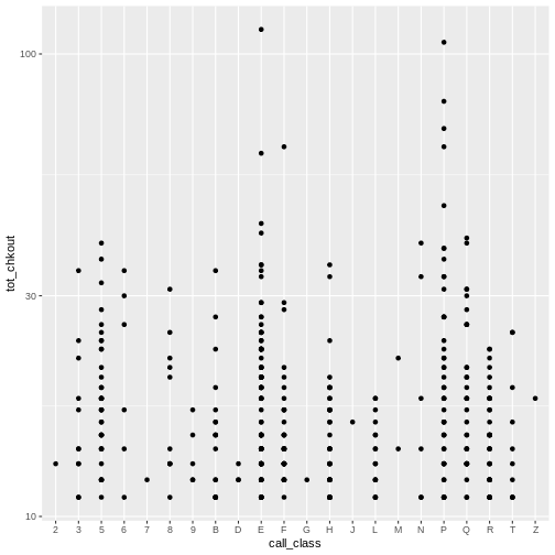
Again, notice the scale on the y axis. We can obseve a few items of
interest here: No items in the D, J, M, and Z class have more than 30
checkouts. An item in the E class has the most checkouts with over 100,
but, as noted above, this includes Easy books classified with
E, not just items with Library of Congress E
classification (United States history) an issue we’ll look at further
down.
Just as with univariate plots, we can use different geoms to view various aspects of the data, which in turn reveal different patterns.
R
# boxplot plot high usage books by call number class
ggplot(data = booksHighUsage,
       aes(x = call_class, y = tot_chkout)) +
  geom_boxplot() +
  scale_y_log10()
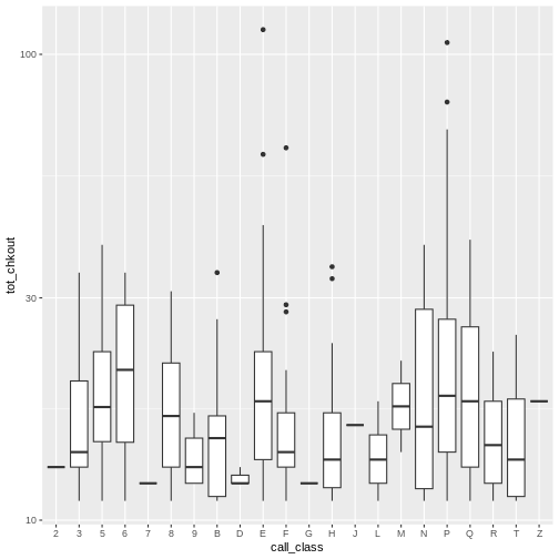
By adding points to a boxplot, we can have a better idea of the
number of measurements and of their distribution. Here we set the
boxplot alpha to 0, which will make it
see-through. We also add another layer of geom to the plot called
geom_jitter(), which will introduce a little bit of
randomness into the position of our points. We set the
color of these points to "tomato".
R
ggplot(data = booksHighUsage, aes(x = call_class, y = tot_chkout)) +
  geom_boxplot(alpha = 0) +
  geom_jitter(alpha = 0.5, color = "tomato") +
  scale_y_log10()
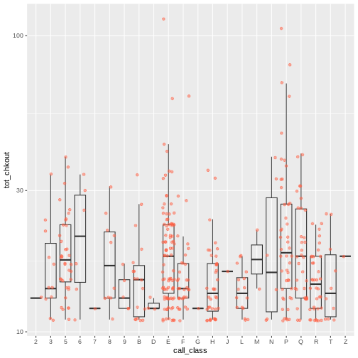
Notice how the boxplot layer is behind the jitter layer? What do you need to change in the code to put the boxplot in front of the points such that it’s not hidden?
Plotting Exercise
Boxplots are useful summaries, but hide the shape of the distribution. For example, if the distribution is bimodal, we would not see it in a boxplot. An alternative to the boxplot is the violin plot, where the shape (of the density of points) is drawn.
- Replace the box plot with a violin plot; see
geom_violin().
R
ggplot(data = booksHighUsage, aes(x = call_class, y = tot_chkout)) +
  geom_violin(alpha = 0) +
  geom_jitter(alpha = 0.5, color = "tomato")
WARNING
Warning: Groups with fewer than two data points have been dropped.
Groups with fewer than two data points have been dropped.
Groups with fewer than two data points have been dropped.
Groups with fewer than two data points have been dropped.
Groups with fewer than two data points have been dropped.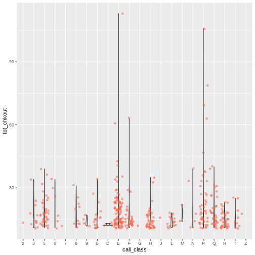
R
ggplot(data = booksHighUsage, aes(x = call_class, y = tot_chkout)) +
geom_violin(alpha = 0) +
geom_jitter(alpha = 0.5, aes(color = subCollection)) +
scale_y_log10()
WARNING
Warning: Groups with fewer than two data points have been dropped.
Groups with fewer than two data points have been dropped.
Groups with fewer than two data points have been dropped.
Groups with fewer than two data points have been dropped.
Groups with fewer than two data points have been dropped.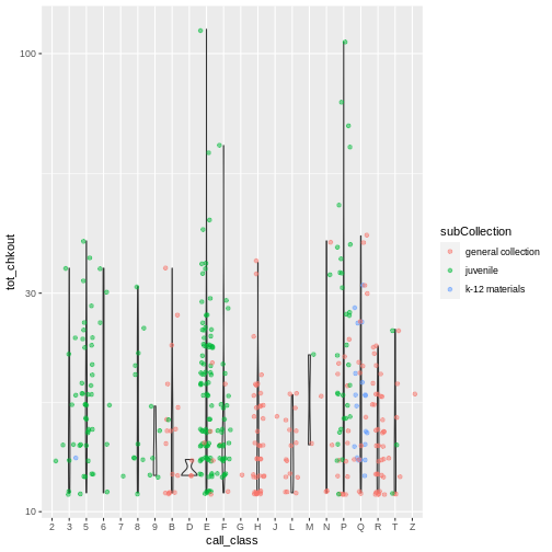
Plotting Exercise(continued)
So far, we’ve looked at the distribution of checkouts within call number ranges. Try making a new plot to explore the distribution of checkouts within another variable.
- Still using the
booksHighUsagedata, create a boxplot fortot_chkoutfor eachsubCollection. Overlay the boxplot layer on a jitter layer to show actual measurements. Keep thescale_y_log10argument.
R
ggplot(data = booksHighUsage, aes(x = subCollection, y = tot_chkout)) +
 geom_boxplot(alpha = 0) +
 geom_jitter(alpha = 0.5, color = "tomato") +
 scale_y_log10()
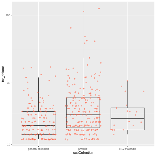
Add a third variable
As we saw in that exercise, you can convey even more information in your visualization by adding a third variable, in addition to the first two on the x and y scales.
Add a third variable with aes()
We can use arguments in aes() to map a visual aesthetic
in the plot to a variable in the dataset. Specifically, we will map
color to the subCollection variable. Because
we are now mapping features of the data to a color, instead of setting
one color for all points, the color now needs to be set inside a call to
the aes function.
ggplot2 will provide a different color
corresponding to different values in the vector. In other words,
associate the name of the aesthetic (color) to the name of
the variable (subCollection) inside aes():
R
ggplot(data = booksHighUsage,
       aes(x = call_class,
           y = tot_chkout,
           color = subCollection)) +
  geom_point() +
  scale_y_log10()
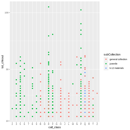
ggplot() automatically assigns a unique level of the
aesthetic to each unique value of the variable (this is called
scaling). Now we reveal indeed that youth materials make up a
large number of high usage items in both the E and the P class.
Use fill() with geom_bar() to create a
stacked bar plot to visualize frequency. Again, this reinforced the fact
that most of the E and P classification are
youth materials.
R
ggplot(data = booksHighUsage, aes(x = call_class)) +
  geom_bar(aes(fill = subCollection))
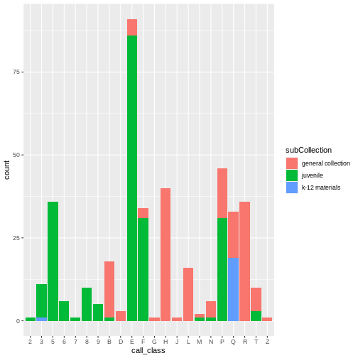
Stacked bar charts are generally more difficult to read than
side-by-side bars. We can separate the portions of the stacked bar that
correspond to each village and put them side-by-side by using the
position argument for geom_bar() and setting
it to “dodge”.
R
ggplot(data = booksHighUsage, aes(x = call_class)) +
  geom_bar(aes(fill = subCollection), position = "dodge")
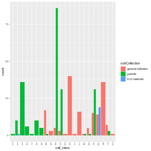
The order of the classification scale is sorted for “library order.”
The audience of library professionals typically prefer an alphabetical
arrangement. However, the x-axis variable is actually categorical.
Categorical data are easier to read when the bars are sorted by
frequency. An easy way to sort by frequency is to use the
fct_infreq() function from the forcats
library.
R
ggplot(data = booksHighUsage, aes(x = fct_infreq(call_class))) +
  geom_bar()
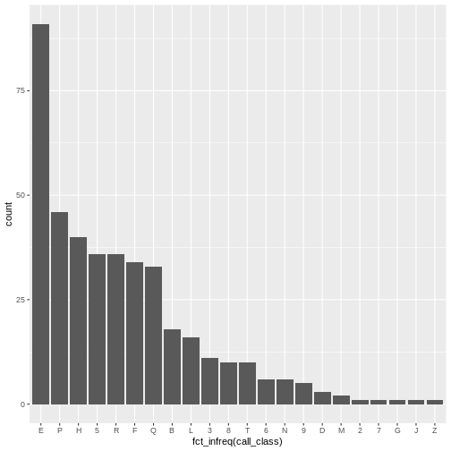
Another visualization issue is labeling. In many cultures, long
labels are easier to read horizontally. Our goal is to flip the x-axis
and reorient the x-axis labels into a horizontal presentation. To
accomplish this, flip the axis coordinates with the
coord_flip() function. When we flip the axes it’s important
to reverse the sorted categorical order. Do this with
forcats::fct_rev().
R
ggplot(data = booksHighUsage, aes(x = fct_rev(fct_infreq(call_class)))) +
  geom_bar() +
  coord_flip()
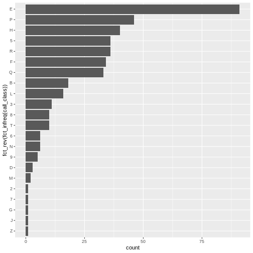
Plotting time series data
Let’s calculate number of counts per year for each format for items
published after 1990 and before 2002 in the booksHighUsage
data frame created above.
First, we use the ymd() function from the
lubridate package to convert our publication year into a
POSIXct object. Pass the truncated = 2 argument as
a way to indicate that the pubyear column does not contain
month or day. This means 1990 becomes
1990-01-01. This will allow us to plot the number of books
per year.
We will do this by calling mutate() to create a new
variable pubyear_ymd.
R
booksPlot <- booksPlot %>%
  mutate(pubyear_ymd = ymd(pubyear, truncated = 2))  # convert pubyear to a Date object with ymd()

class(booksPlot$pubyear)  # integer
OUTPUT
[1] "numeric"R
class(booksPlot$pubyear_ymd) # Date
OUTPUT
[1] "Date"Next we can use filter to remove the NA
values and get books published between 1990 and 2003. Notice that we use
the & as an AND operator to indicate that the date must
fall between that range. We then need to group the data and count
records within each group.
R
yearly_counts <- booksPlot %>%
  filter(!is.na(pubyear_ymd),
         pubyear_ymd > "1989-01-01" & pubyear_ymd < "2002-01-01") %>%
  count(pubyear_ymd, subCollection)
Time series data can be visualized as a line plot with years on the x axis and counts on the y axis:
R
ggplot(data = yearly_counts, mapping = aes(x = pubyear_ymd, y = n)) +
     geom_line()

Unfortunately, this does not work because we plotted data for all the
sub-collections together. We need to tell ggplot to draw a line for each
sub-collection by modifying the aesthetic function to include
group = subCollection:
R
ggplot(data = yearly_counts, mapping = aes(x = pubyear_ymd, y = n, group = subCollection)) +
    geom_line()
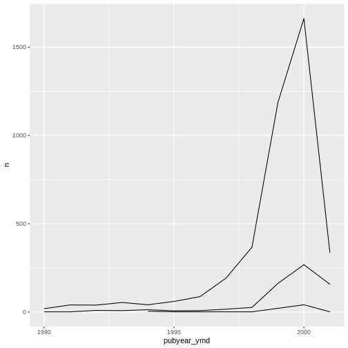
We will be able to distinguish sub-collections in the plot if we add
colors (using color also automatically groups the
data):
R
ggplot(data = yearly_counts, mapping = aes(x = pubyear_ymd, y = n, color = subCollection)) +
  geom_line()
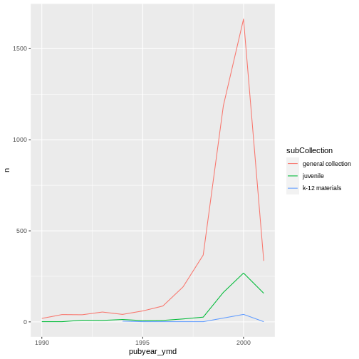
Add a third variable with facets
Rather than creating a single plot with side-by-side bars for each sub-collection, we may want to create multiple plots, where each plot shows the data for a single sub-collection. This would be especially useful if we had a large number of sub-collections that we had sampled, as a large number of side-by-side bars will become more difficult to read.
ggplot2 has a special technique called
faceting that allows the user to split one plot into multiple
plots based on a factor included in the dataset.
There are two types of facet functions:
-
facet_wrap()arranges a one-dimensional sequence of panels to allow them to cleanly fit on one page. -
facet_grid()allows you to form a matrix of rows and columns of panels.
Both geometries allow to to specify faceting variables specified
within vars(). For example,
facet_wrap(facets = vars(facet_variable)) or
facet_grid(rows = vars(row_variable), cols = vars(col_variable)).
Here we use facet_wrap() to make a time series plot for
each subCollection
R
ggplot(data = yearly_counts, mapping = aes(x = pubyear_ymd, y = n)) +
    geom_line() +
    facet_wrap(facets = vars(subCollection))
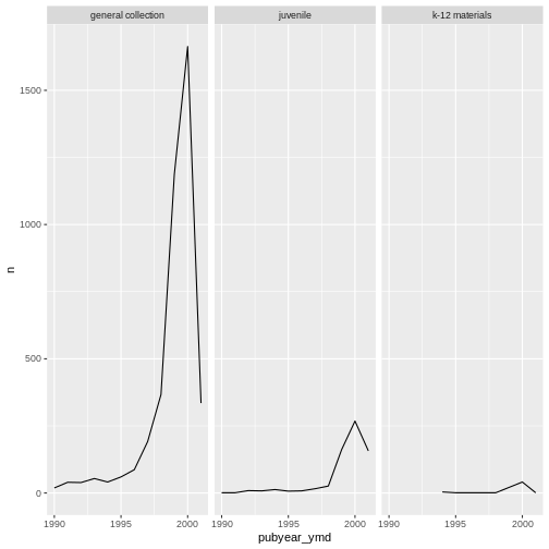
We can use facet_wrap() as a way of seeing the
categories within a variables. Look at the number of formats per
sub-collection.
R
ggplot(data = books2, aes(x = fct_rev(fct_infreq(subCollection)))) +
  geom_bar() +
  facet_wrap(~ format, nrow = 2) +
  scale_y_log10() +
  coord_flip() +
  labs(x = "Library subcollection", y = "")
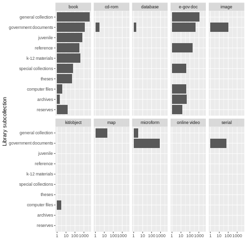
While this may not be the most beautiful plot, these kinds of exercises can be helpful for data exploration. We learn that there are books in all sub-collections; there are CD-ROMS, serials, images, and microforms in government documents, and so on. Exploratory plots visually surface information about your data that are otherwise difficult to parse. Sometimes they may not meet all the rules for creating beautiful data, but when you are simply getting to know your data, that’s OK.
Challenge
Use the books2 data to create a bar plot that depicts
the number of items in each sub-collection, faceted by format. Add the
scale_y_log10() argument to create a logarithmic scale for easier
visibility. Add the following theme argument to tilt the axis text
diagonal:
theme(axis.text.x = element_text(angle = 60, hjust = 1))
R
ggplot(data = books2, aes(x = subCollection)) +
geom_bar() +
facet_wrap(vars(format)) +
scale_y_log10() +
theme(axis.text.x = element_text(angle = 60, hjust = 1))
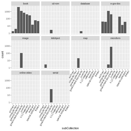
ggplot2 themes
Usually plots with white background look more readable when printed.
Every single component of a ggplot graph can be customized
using the generic theme() function. However, there are
pre-loaded themes available that change the overall appearance of the
graph without much effort.
For example, we can change our graph to have a simpler white
background using the theme_bw() function:
R
#
ggplot(data = yearly_counts, mapping = aes(x = pubyear_ymd, y = n)) +
  geom_line() +
  facet_wrap(facets = vars(subCollection)) +
  theme_bw()
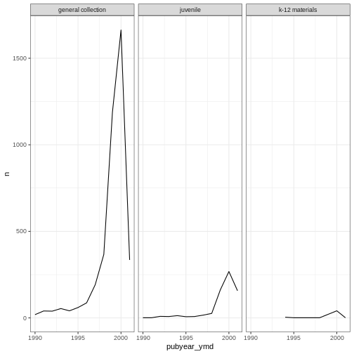
In addition to theme_bw(), which changes the plot
background to white, ggplot2 comes with
several other themes which can be useful to quickly change the look of
your visualization. The complete list of themes is available at https://ggplot2.tidyverse.org/reference/ggtheme.html.
theme_minimal() and theme_light() are popular,
and theme_void() can be useful as a starting point to
create a new hand-crafted theme.
The ggthemes
package provides a wide variety of options. The ggplot2
extensions website provides a list of packages that extend the
capabilities of ggplot2, including
additional themes.
Customization
Take a look at the ggplot2
cheat sheet, and think of ways you could improve your plots.
For example, by default, the axes labels on a plot are determined by the name of the variable being plotted. We can change names of axes to something more informative than ‘pubyear_ymd’ and ‘n’ and add a title to the figure:
R
# add labels
ggplot(data = yearly_counts, mapping = aes(x = pubyear_ymd, y = n)) +
  geom_line() +
  facet_wrap(facets = vars(subCollection)) +
  theme_bw() +
    labs(title = "Number of High Usage Books per Year of Publication, by Sub-Collection",
        x = "Year of publication",
        y = "Number of books")
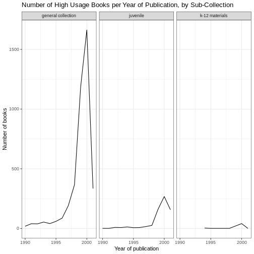
Note that it is also possible to change the fonts of your plots. If
you are on Windows, you may have to install the extrafont
package, and follow the instructions included in the README for this
package.
You can also assign a theme to an object in your
environment, and pass that theme to your plot. This can be helpful to
keep your ggplot() calls less cluttered. Here we create a
gray_theme :
R
# create the gray theme
gray_theme <- theme(axis.text.x = element_text(color = "gray20", size = 12, angle = 45, hjust = 0.5, vjust = 0.5),
                    axis.text.y = element_text(color = "gray20", size = 12),
                    text = element_text(size = 16),
                    plot.title = element_text(hjust = 0.5))

# pass the gray theme to a plot
ggplot(data = yearly_counts, mapping = aes(x = pubyear_ymd, y = n)) +
  geom_line() +
  facet_wrap(facets = vars(subCollection)) +
  gray_theme +
  labs(title = "Number of High Usage Books per Year of Publication, \n by Sub-Collection",
        x = "Year of publication",
        y = "Number of books")
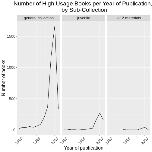
Challenge
Use the booksPlot data to create a plot that depicts how
the total number of checkouts changes based on year of publication.
First, create a data frame yearly_checkouts That meets
the following conditions:
-
filter()to excludeNAvalues -
filter()between “1989-01-01” and “2002-01-01” -
group_by()the publication year (make sure to use the special Date pubyear value we created) -
summarize()to create a new valuecheckouts_sumthat represents thesum()of total checkouts per publication year
Then, create a ggplot that visualizes the sum of item
checkouts by year of publication. Add one of the themes listed
above.
R
yearly_checkouts <- booksPlot %>%
 filter(!is.na(pubyear_ymd),
        pubyear_ymd > "1989-01-01" & pubyear_ymd < "2002-01-01") %>%
 group_by(pubyear_ymd) %>%
 summarize(checkouts_sum = sum(tot_chkout))

ggplot(data = yearly_checkouts, mapping = aes(x = pubyear_ymd, y = checkouts_sum)) +
 geom_line() +
 theme_bw()
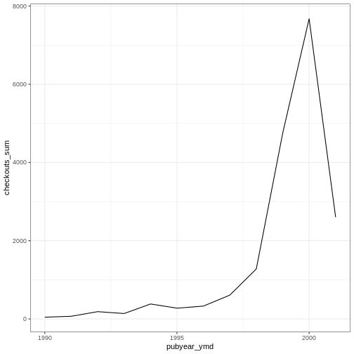
Save and export
After creating your plot, you can save it to a file in your favorite format. The Export tab in the Plot pane in RStudio will save your plots at low resolution, which will not be accepted by many journals and will not scale well for posters.
Instead, use the ggsave() function, which allows you
easily change the dimension and resolution of your plot by adjusting the
appropriate arguments (width, height and
dpi). We have been printing our plot output directly to the
console. To use ggsave(), first assign the plot to a
variable in your R environment, such as
yearly_counts_plot.
Make sure you have the fig_output/ folder in your
working directory.
R
yearly_counts_plot <- ggplot(data = yearly_counts, mapping = aes(x = pubyear_ymd, y = n)) +
  geom_line() +
  facet_wrap(facets = vars(subCollection)) +
  gray_theme +
  labs(title = "Number of High Usage Books per Year of Publication, \n by Sub-Collection",
        x = "Year of publication",
        y = "Number of books")

ggsave("fig_output/yearly_counts_plot.png", yearly_counts_plot, width = 15, height = 10)
Exercise
With all of this information in hand, please take another five
minutes to either improve one of the plots generated in this exercise or
create a beautiful graph of your own. Use the RStudio ggplot2
cheat sheet for inspiration. Here are some ideas:
- See if you can make the bars white with black outline.
- Try using a different color palette (see http://www.cookbook-r.com/Graphs/Colors_(ggplot2)/).
Key Points
-
ggplot2is a flexible and useful tool for creating plots in R. - The data set and coordinate system can be defined using the
ggplotfunction. - Additional layers, including geoms, are added using the
+operator. - Boxplots are useful for visualizing the distribution of a continuous variable.
- Barplot are useful for visualizing categorical data.
- Faceting allows you to generate multiple plots based on a categorical variable.
Comments
All programming languages allow the programmer to include comments in their code. To do this in R we use the
#character. Anything to the right of the#sign and up to the end of the line is treated as a comment and will not be evaluated by R. You can start lines with comments or include them after any code on the line.Comments are essential to helping you remember what your code does, and explaining it to others. Commenting code, along with documenting how data is collected and explaining what each variable represents, is essential to reproducible research. See the Software Carpentry lesson on R for Reproducible Scientific Analysis.
R
OUTPUT
RStudio makes it easy to comment or uncomment a paragraph: after selecting the lines you want to comment, press at the same time on your keyboard Ctrl + Shift + C. If you only want to comment out one line, you can put the cursor at any location of that line (i.e. no need to select the whole line), then press Ctrl + Shift + C.