Python for Librarians

Starting With Data

Overview

Teaching: ?? min
Exercises: ?? min

Questions

How does Python deal with data tables?

Objectives

Explain what a library is, and what libraries are used for.

Load a Python/Pandas library.

Read tabular data from a file into Python using Pandas using read_csv.

Learn about the Pandas DataFrame object.

Learn about data slicing and indexing.

Perform mathematical operations on numeric data.

Create simple plots of data.

Working with Pandas DataFrames in Python

Presentation of the DOAJ Articles data

For this lesson, we will be using Directory of Open Access Journals (DOAJ) article sample data, available on FigShare. Download this zip and extract it on your working directory on a meaningful location (e.g. create a folder called data/)

This data set is a list of published articles. The dataset is stored as .csv (comma separated values) files: each row holds information for a single article, and the columns represent:

Column	Description
Title	Title of the article
Authors	Author (or authors)
DOI	DOI
URL	URL
Subjects	List of subject key words
ISSNs	ISSNs code
Citation	Citation information
LanguageId	Language identifier
LicenceId	License identifier
Author_Count	Number of authors of the article
First_Author	Name of the first author
Citation_Count	Number times it has been cited
Day	Day of publication
Month	Month of publication
Year	Year of publication

About (Software) Libraries

A library in Python contains a set of tools (called functions) that perform tasks on our data. Importing a library is like getting a piece of lab equipment out of a storage locker and setting it up on the bench for use in a project. Once a library is set up, it can be used or called to perform many tasks.

Pandas in Python

One of the best options for working with tabular data in Python is to use the pandas data analysis library. Pandas provides data structures, produces high quality plots with matplotlib, and integrates nicely with other libraries that use NumPy (which is another Python library) arrays.

Python doesn’t load all of the libraries available to it by default. We have to add an import statement to our code in order to use library functions. To import a library, we use the syntax import libraryName. If we want to give the library a nickname to shorten the command, we can add as nickNameHere. An example of importing the pandas library using the common nickname pd is below.

import pandas as pd

Each time we call a function that’s in a library, we use the syntax LibraryName.FunctionName. Adding the library name with a . before the function name tells Python where to find the function. In the example above, we have imported Pandas as pd. This means we don’t have to type out pandas each time we call a Pandas function.

Lesson Overview

For this lesson we will be using the Directory of Open Access Journals (DOAJ) article data.

We are analyzing the articles published in a particular field of study. The data set is stored in .csv (comma separated values) format. Within the .csv files, each row holds information for a single article.

The first few rows of our first file (articles.csv) look like this:

id,Title,Authors,DOI,URL,Subjects,ISSNs,Citation,LanguageId,LicenceId,Author_Count,First_Author,Citation_Count,Day,Month,Year
0,The Fisher Thermodynamics of Quasi-Probabilities,Flavia Pennini|Angelo Plastino,10.3390/e17127853,https://doaj.org/article/b75e8d5cca3f46cbbd63e91be5b32412,Fisher information|quasi-probabilities|complementarity|Physics|QC1-999|Science|Q,1099-4300,"Entropy, Vol 17, Iss 12, Pp 7848-7858 (2015)",1,1,2,Flavia Pennini,4,1,11,2015
1,Aflatoxin Contamination of the Milk Supply: A Pakistan Perspective,Naveed Aslam|Peter C. Wynn,10.3390/agriculture5041172,https://doaj.org/article/0edc5af6672641c0bd45608812a34f9e,aflatoxins|AFM1|AFB1|milk marketing chains|hepatocellular carcinoma|Agriculture (General)|S1-972|Agriculture|S,2077-0472,"Agriculture (Basel), Vol 5, Iss 4, Pp 1172-1182 (2015)",1,1,2,Naveed Aslam,5,1,11,2015
2,Metagenomic Analysis of Upwelling-Affected Brazilian Coastal Seawater Reveals Sequence Domains of Type I PKS and Modular NRPS,Rafael R. C. Cuadrat|Juliano C. Cury|Alberto M. R. Dávila,10.3390/ijms161226101,https://doaj.org/article/d9fe469f75a0442382b84ba4f50007ee,PKS|NRPS|metagenomics|environmental genomics|upwelling|coastal environment|Chemistry|QD1-999|Science|Q,1422-0067,"International Journal of Molecular Sciences, Vol 16, Iss 12, Pp 28285-28295 (2015)",1,1,3,Rafael R. C. Cuadrat,8,1,11,2015
3,"Synthesis and Reactivity of a Cerium(III) Scorpionate Complex Containing a Redox Non-Innocent 2,2′-Bipyridine Ligand",Fabrizio Ortu|Hao Zhu|Marie-Emmanuelle Boulon|David P. Mills,10.3390/inorganics3040534,https://doaj.org/article/95606ed39deb4f43b96f7e6308ad15d3,lanthanide|cerium|scorpionate|tris(pyrazolyl)borate|radical|redox non-innocent|Inorganic chemistry|QD146-197,2304-6740,"Inorganics (Basel), Vol 3, Iss 4, Pp 534-553 (2015)",1,1,4,Fabrizio Ortu,5,1,11,2015

(quite difficult to read and interpret as it is…)

We want to:

Load that data into memory using Python.
Calculate the average number of authors per article, for each publisher.
Plot this information.

We can automate the process above using Python. It is efficient to spend time building the code to perform these tasks because once it is built, we can use it over and over on different datasets that use a similar format. This makes our methods easily reproducible. We can also easily share our code with colleagues and they can replicate the same analysis.

Reading CSV data using Pandas

We will begin by locating and reading our survey data which are in CSV format (comma separated values). We can use Pandas’ read_csv function to pull the file directly into a DataFrame.

So what’s a DataFrame?

A DataFrame is a 2-dimensional data structure that can store data of different types (including characters, integers, floating point values, factors and more) in columns. It is similar to a spreadsheet or an SQL table or the data.frame in R. A DataFrame always has an index (0-based). An index refers to the position of an element in the data structure.

First, let’s make sure the Python Pandas library is loaded. We will import Pandas using the nickname pd. This is a common convention on the internet, so if you look up Pandas usage, you will often see it this way.

import pandas as pd

Let’s also import the OS Library. This library allows us to make sure we are in the correct working directory. If you are working in IPython or Jupyter Notebook, be sure to start the notebook in the workshop repository. If you didn’t do that you can always set the working directory using the code below.

import os
os.getcwd()
# if this directory isn't right, use the command below to set the working directory
os.chdir("YOURPathHere")

# note that pd.read_csv is used because we imported pandas as pd
pd.read_csv("articles.csv")

The above command yields the output below:

        id                                              Title  \
      0   The Fisher Thermodynamics of Quasi-Probabilities   
      1  Aflatoxin Contamination of the Milk Supply: A ...   
      2  Metagenomic Analysis of Upwelling-Affected Bra...   
      3  Synthesis and Reactivity of a Cerium(III) Scor...   
...
  997  Crystal structure of bis(3-bromopyridine-κN)bi...   
  998  Crystal structure of 4,4′-(ethane-1,2-diyl)bis...   
  999  Crystal structure of (Z)-4-[1-(4-acetylanilino...   
1000  Metagenomic Analysis of Upwelling-Affected Bra...

...

      Month  Year  
      11  2015  
      11  2015  
      11  2015  
...
     1  2015  
     1  2015  
   11  2015  

[1001 rows x 16 columns]

We can see that there were 1,001 rows parsed. Each row has 11 columns. The first column is the index of the DataFrame. The index is used to identify the position of the data, but it is not an actual column of the DataFrame. It looks like the read_csv function in Pandas read our file properly. However, we haven’t saved any data to memory so we can work with it. We need to assign the DataFrame to a variable. Remember that a variable is a name for a value, such as x, or data. We can create a new object with a variable name by assigning a value to it using =.

Let’s call the imported survey data articles_df:

articles_df = pd.read_csv("articles.csv")

Notice when you assign the imported DataFrame to a variable, Python does not produce any output on the screen. We can print the value of the articles_df object by typing its name into the Python command prompt.

articles_df

which prints contents like above.

Manipulating our Articles data

Now we can start manipulating our data. First, let’s check the data type of the data stored in articles_df using the type method. The type method and __class__ attribute tell us that articles_df type is <class 'pandas.core.frame.DataFrame'>.

type(articles_df)
# this does the same thing as the above!
articles_df.__class__

<class 'pandas.core.frame.DataFrame'>

We can also enter articles_df.dtypes at our prompt to view the data type for each column in our DataFrame.

int64 represents numeric integer values (int64 cells can not store decimals).
object represents strings (letters and numbers).
float64 represents numbers with decimals.

articles_df.dtypes

which returns:

id                 int64
Title             object
Authors           object
DOI               object
URL               object
Subjects          object
ISSNs             object
Citation          object
LanguageId         int64
LicenceId          int64
Author_Count       int64
First_Author      object
Citation_Count     int64
Day                int64
Month              int64
Year               int64
dtype: object

We’ll talk a bit more about what the different data types mean later in Data Types and Formats.

Useful ways to view DataFrame objects in Python

There are multiple methods that can be used to summarize and access the data stored in DataFrames. Let’s try out a few. Note that we call the method by using the object name articles_df.method. So articles_df.columns provides an index of all of the column names in our DataFrame.

Try out the methods below to see what they return.

articles_df.columns

articles_df.head() - Also, what does articles_df.head(15) do?

articles_df.tail()

articles_df.shape - Take note of the output of the shape method. What format does it return the shape of the DataFrame in?

HINT: More on tuples, here.

Calculating statistics from data in a Pandas DataFrame

We’ve read our data into Python. Next, let’s perform some quick summary statistics to learn more about the data that we’re working with. We can perform summary stats quickly using groups. But first we need to figure out what we want to group by.

Let’s begin by exploring our data:

# Look at the column names
articles_df.columns.values

which returns:

array(['id', 'Title', 'Authors', 'DOI', 'URL', 'Subjects', 'ISSNs',
       'Citation', 'LanguageId', 'LicenceId', 'Author_Count',
       'First_Author', 'Citation_Count', 'Day', 'Month', 'Year'], dtype=object)

Let’s get a list of all the months that articles were published in. The pd.unique function tells us all of the unique values in a column.

pd.unique(articles_df['Month'])

which returns:

array([11, 12,  8,  4, 10,  9,  7,  6,  5,  3,  2,  1])

Which show us that articles have been published in every month of the year.

Challenge

Create a list of unique ISSNs found in the articles data. Call it publications (Note: each publication has a unique ISSN). How many unique publications (ISSNs) are there in the data?

Groups in Pandas

Our DataFrame has a mixture of String and Numeric types. Some of the grouping operations work different for numeric types (e.g. calculating averages).

We often want to calculate summary statistics grouped by subsets or attributes within fields of our data. For example, we might want to know the number of articles published in each publication.

We can calculate basic statistics for all records in a single column using the syntax below:

articles_df['Citation_Count'].describe()

gives:

count    1001.000000
mean        9.023976
std         1.655121
min         3.000000
25%         9.000000
50%        10.000000
75%        10.000000
max        10.000000
Name: Citation_Count, dtype: float64

We can also extract one specific metric if we wish:

articles_df['ISSNs'].unique()
articles_df['ISSNs'].count()

articles_df['Citation_Count'].min()
articles_df['Citation_Count'].max()
articles_df['Citation_Count'].mean()
articles_df['Citation_Count'].std()

But if we want to summarize by one or more variables, for example Language, we can use Pandas’ .groupby method. Once we’ve created a groupby DataFrame, we can quickly calculate summary statistics by a group of our choice.

# Group data by Language
byLang = articles_df.groupby('LanguageId')

The Pandas function describe will return descriptive stats including: mean, median, max, min, std and count for a particular column in the data. Pandas’ describe function will only return summary values for columns containing numeric data.

# summary statistics for all numeric columns by Language
byLang.describe()
# provide the mean for each numeric column by Language
byLang.mean()

gives this output:

                    id  LicenceId  Author_Count  Citation_Count  Day  \
LanguageId                                                             
1           510.004090   1.052147      4.013292        9.137014  1.0   
2            52.533333   1.000000      3.333333        4.333333  1.0   
3           116.571429   4.000000      4.142857        4.000000  1.0   
4           112.000000   4.000000      5.000000        4.000000  1.0   

                Month    Year  
LanguageId                     
1            6.332311  2015.0  
2           11.000000  2015.0  
3           12.000000  2015.0  
4           12.000000  2015.0  

The groupby command is powerful in that it allows us to quickly generate summary stats.

Challenge
How many articles are published in each publication?
What happens when you group by two columns using the following syntax and then grab mean values:
byMultiple = articles_df.groupby(['LanguageId', 'ISSNs'])
byMultiple.mean()
Summarize author counts for each publication (ISSNs) in your data. HINT: you can use the following syntax to only create summary statistics for one column in your data by_ISSNs['Author_Count'].describe()

Did you get it right?

The Output from question 3 of the previous challenge looks like this:

ISSNs                     
0367-0449|1988-3250  count    11.000000
                     mean      4.000000
                     std       2.720294
                     min       2.000000
                     25%       2.000000
                     50%       3.000000
                     75%       5.000000
                     max       9.000000
1099-4300            count     1.000000
...

Quickly creating summary counts in Pandas

Let’s next count the number of articles for each publisher. We can do this in a few ways, but we’ll use groupby combined with a count() method.

# count the number of samples by publisher
article_counts = articles_df.groupby('ISSNs')['Title'].count()

Or, we can also count just the rows that have the ISSN “1420-3049”:

articles_df.groupby('ISSNs')['Title'].count()['1420-3049']

Basic Math functions

If we wanted to, we could perform math on an entire column of our data. For example let’s multiply all author count values by 2. A more practical use of this might be to normalize the data according to a mean, area, or some other value calculated from our data.

# multiply all author count values by 2
articles_df['Author_Count'] * 2

Another Challenge

What’s another way to create a list of licenses and associated count of the records in the data? Hint: you can perform count, min, etc functions on groupby DataFrames in the same way you can perform them on regular DataFrames.

Quick & easy plotting data using Pandas

We can plot our summary stats using Pandas, too.

# make sure figures appear inline in Ipython Notebook
%matplotlib inline
# create a quick bar chart
article_counts.plot(kind='bar')

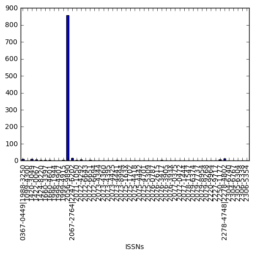Articles by ISSN plot

We can also look at how many articles were published in each language:

language_count = articles_df.groupby('LanguageId')['Title'].count()
# let's plot that too
language_count.plot(kind='bar');

Activities

Create a plot of average number of authors across all publishers.

Create a plot of average number of authors across all publishers per language.

Summary Plotting Challenge

Create a stacked bar plot, with Number of articles on the Y axis, and the stacked variable being LicenceId. The plot should show total number of articles by license for each month. Some tips are below to help you solve this challenge:

For more on Pandas plots, visit this link.

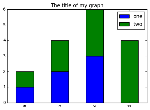
You can use the code that follows to create a stacked bar plot but the data to stack need to be in individual columns. Here’s a simple example with some data where ‘a’, ‘b’, and ‘c’ are the groups, and ‘one’ and ‘two’ are the subgroups.
d = {'one' : pd.Series([1., 2., 3.], index=['a', 'b', 'c']),'two' : pd.Series([1., 2., 3., 4.], index=['a', 'b', 'c', 'd'])}
pd.DataFrame(d)
shows the following data
       one  two
   a    1    1
   b    2    2
   c    3    3
   d  NaN    4
We can plot the above with
# plot stacked data so columns 'one' and 'two' are stacked
my_df = pd.DataFrame(d)
my_df.plot(kind='bar',stacked=True,title="The title of my graph")
You can use the .unstack() method to transform grouped data into columns for each plotting. Try running .unstack() on some DataFrames above and see what it yields.

Start by transforming the grouped data (by LicenceId and Month) into an unstacked layout, then create a stacked plot.

Solution to Summary Challenge

First we group data by Month and by LicenceId, and then calculate a total for each Month.
by_month_lic = articles_df.groupby(['Month','LicenceId'])
month_lic_count = by_month_lic.size()
This calculates the number of articles for each Month and LicenceId as a table
Month  LicenceId
1      1             50
2      1             96
3      1             79
4      1             69
       2              7
5      1            107
6      1             91
7      1             94
8      1             90
       2             13
9      1             77
10     1            104
11     1             97
       2             10
       3              6
12     4             11
dtype: int64
Below we’ll use .unstack() on our grouped data to figure out the total weight that each language contributed to each publisher.
by_month_lic = articles_df.groupby(['Month','LicenceId'])
month_lic_count = by_month_lic.size()
mlc = month_lic_count.unstack()
The unstack function above will display the following output:
LicenceId   1    2    3    4
Month
1          50  NaN  NaN  NaN
2          96  NaN  NaN  NaN
3          79  NaN  NaN  NaN
4          69    7  NaN  NaN
5         107  NaN  NaN  NaN
6          91  NaN  NaN  NaN
7          94  NaN  NaN  NaN
8          90   13  NaN  NaN
9          77  NaN  NaN  NaN
10        104  NaN  NaN  NaN
11         97   10    6  NaN
12        NaN  NaN  NaN   11
Now, create a stacked bar plot with that data where the article count for each Month are stacked by License.

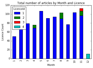
Rather than display it as a table, we can plot the above data by stacking the values of each licence as follows:
by_month_lic = articles_df.groupby(['Month','LicenceId'])
month_lic_count = by_month_lic.size()
mlc = month_lic_count.unstack()

s_plot = mlc.plot(kind='bar',stacked=True,title="Total number of articles by Month and Licence")
s_plot.set_ylabel("Licence Count")
s_plot.set_xlabel("Month");

Key Points

Core concepts in python: Python libraries, Pandas DataFrames, working with data.